Deep Learning Notes

Introduction to Generative AI - Coursera

Generative AI can input only one modality and output multiple modalities.

DL can process more complex patterns than traditional ML.

$y = f(x)$ | $x$ is input data, $y$ is model output and $f$ is model.

Pre-Training: 1) Large amount of data; 2) Billions of parameters; 3) Unsupervised Learning

Transformer Challenges: 1) The model is not trained on enough data; 2) is trained on noisy or dirty data; 3) is not given enough context; 4) is not given enough constraints.

Prompt is given to the LLMs as input and it can be used to control the output of the model. (The quality of the input determines the quality of the output)

Hung-yi Lee 2021 Spring ML

1. Introduction

对一个模型的修改往往基于对问题的理解，也就是 domain knowledge

ML Framework (3 Steps)

Function with Unknown: $y = b + wx_1$, $w$ and $b$ are unknown parameters (weight and bias), $x_1$ is feature. $\leftarrow$ Linear Model
Define Loss Function from Training Data: is a function of parameters $L(b, w)$, $L = \frac{1}{N} \sum_{n}^{}e_n$ and is from training data.

MAE (Mean Absolute Error): $e = \vert y - \hat{y} \vert$

MSE (Mean Square Error): $e = (y - \hat{y})^2$
Optimization: $w^*, b^* = \arg \min\limits_{w, b} L$

Gradient Descent: $w^1 \leftarrow w^0 - \eta\frac{\partial L}{\partial w}\vert_{w = w^0,\ b = b^0}$, $w^0$ is randomly picked and $\eta$ is learning rate (a hyperparameter that dictates the speed at which the model adjusts its parameters during training). If gradient is negative (gradient guides the direction), increase $w$ can decrease loss.

Step into DL

Function with Unknown

sigmoid: $\frac{1}{1 + e^{-x}}$, $y = c \ \frac{1}{1 + e^{-(b + wx_1)}} = c \ \text{sigmoid}(b + wx_1)$ 通过改变 $w$、$b$ 和 $c$（constant），就可以得到各种不同形状的 sigmoid 函数。$w$ changes slopes, $b$ changes shifts and $c$ changes heights.

利用 sigmoid 函数来替代阶跃函数作为非线性函数，可以组合各种不同的 linear model，得到 piecewise linear model，从而可以近似各种不同的 continuous function (non-Linear Model)，即
\[y = b + \sum\limits_i c_i \ \text{sigmoid}(b_i + w_i x_1)\]
如果对于不同的 feature 有不同的权重 $w$，那么公式就会变成
\[y = b + \sum\limits_i c_i \ \text{sigmoid}(b_i + \sum\limits_j{w_{ij} x_j})\]
$i$: no. of sigmoid, $j$: no. of features

用线代的形式可以表示为（Timestamp - 17:23）
\[y = b + \boldsymbol{c^T} \sigma(\boldsymbol{b} + \boldsymbol{WX})\]
$c$ 为 transpose 的原因是：矩阵乘法要求前一个矩阵的列数是后一个矩阵的行数。

Using $\boldsymbol{\theta}$ to represent the unknown parameters $\boldsymbol{W}, \boldsymbol{b}, \boldsymbol{c^T}, b$, so the function with unknown can be written as $f_{\boldsymbol{\theta}}$.

Define Loss Function from Training Data

Loss $L(\boldsymbol{\theta})$ is a function of parameters $\boldsymbol{\theta}$，将训练数据经过 $f_{\boldsymbol{\theta}}$ 得到的输出与 ground truth 比较计算出距离（例如 cross-entropy），将每个样本的距离加起来就作为 loss function $L(\boldsymbol{\theta}) = \sum^N_{n=1}e_n$。
Optimization: 对于 $\boldsymbol{\theta} = \begin{bmatrix}\theta_1\\\theta_2\\\theta_3\\\vdots\end{bmatrix}$，要找到 $\boldsymbol{\theta^*} = \arg \min\limits_{\boldsymbol{\theta}} L$，最终 $f_{\boldsymbol{\theta^*}}$ 就是我们想要的那个 function。对于随机选择的初始值 $\boldsymbol{\theta}^0$，计算出 gradient $\boldsymbol{g} = \nabla{L(\boldsymbol{\theta}^0)}$ 后用 gradient descent 就可以更新所有的参数，即 $\boldsymbol{\theta}^1 \leftarrow \boldsymbol{\theta}^0 - \eta\boldsymbol{g}$，通常不会有所有的训练数据去一次又一次地更新参数，而是将训练数据划分成多个 batch，用每一个 batch 去做每一次的 update（called it iteration），比如第一个 batch 得到一个 loss $L^1$，用这个 loss 计算得到的梯度去更新 $\boldsymbol{\theta}^0$ 得到 $\boldsymbol{\theta}^1$，再用第二个 batch 更新得到 $\boldsymbol{\theta}^2$，以此类推，把所有 batch 都看过一遍后叫做一个 epoch。

Rectified Linear Unit (ReLU): $c\max(0, b + wx_1)$

如果使用 ReLU 代替 sigmoid，需要两个 ReLU 才可以得到一个 hard sigmoid，则
\[y = b + \sum\limits_{2i} c_i \max(0, b_i + \sum\limits_j{w_{ij} x_j})\]
这里的 sigmoid 和 ReLU 在 ML 中被称之为 Activation function

Neuron and Neural Network == hidden layer and Deep Learning

Overfitting: Better on training data, worse on unseen data.

2. DL

Backpropagation

神经网络通常有多层且每层有大量的 neuron，因此它会有上百万个参数，用 Backpropagation 就可以有效地计算这些参数的 gradient

Forward Pass: $z = x_1w_1 + x_2w_2 + b \rightarrow \frac{\partial{z}}{\partial{w}}$
Backward Pass: Function $C$ determines the distance between $\hat{y}$ (prediction value) and $y$ (ground truth). $\frac{\partial{\hat{y}}}{\partial{z}}\frac{\partial{C}}{\partial{\hat{y}}} \rightarrow \frac{\partial{C}}{\partial{z}}$
Then, we will get the gradient of parameter $w$ with respect to Function $C$. $\frac{\partial{z}}{\partial{w}} \times \frac{\partial{C}}{\partial{z}} \rightarrow \frac{\partial{C}}{\partial{w}}$

General Guide

Training: $y = f_{\boldsymbol{\theta}}(\boldsymbol{x}), \ L(\boldsymbol{\theta}), \ \boldsymbol{\theta}^* = \arg \min\limits_{\boldsymbol{\theta}} L$

Testing: $y = f_{\boldsymbol{\theta}^*}(\boldsymbol{x}')$

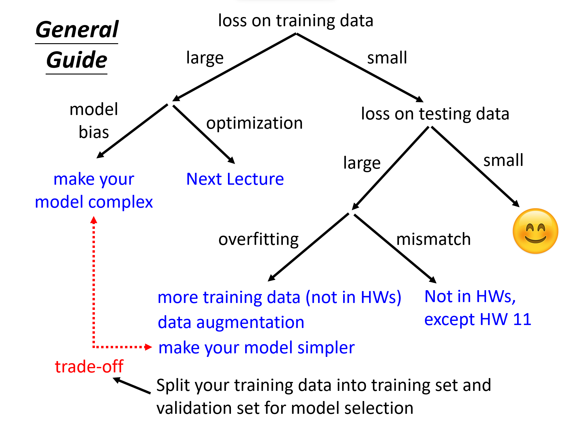
The loss on the training data is important and must be recorded. Before checking the test results, ensure that the loss on the training data is sufficiently small.

Training loss is large
1. Model Bias: model is too simple
  
  Solution: Redesign the model to make it more flexible (more features, more complex architecture)
2. Optimization Issue
  
  Problem: Critical point, Learning rate, Loss function
  
  Solution: More powerful optimization technology, like Mini-batch, Momentum; AdaGrad, RMSProp, Adam, AdamW; Learning rate scheduling; Choose appropriate loss function
  
  Taylor Series Approximation: 能够将任意光滑函数近似为多项式函数，其利用函数在某一点的值及其在该点的所有阶导数来构建一个多项式，这个多项式在该点附近与原函数的值非常接近。
  
  $$ f(x) = f(a) + \frac{f'(a)}{1!}(x-a) + \frac{f''(a)}{2!}(x-a)^2 + \frac{f'''(a)}{3!}(x-a)^3 + \cdots \ or \ f(x) = \sum_{n=0}^{\infty} \frac{f^{(n)}(a)}{n!}(x-a)^n $$
  
  Hessian Matrix: 对于一个高维函数 $f(x_1, x_2, \ldots, x_n)$，矩阵中将包含所有变量对之间的二阶偏导数，即对于 $i$ 个 row 和 $j$ 个 column 的 $x_i$ 和 $x_j$ 来说：
  \[H = \begin{bmatrix} \frac{\partial^2 f}{\partial x_1^2} & \frac{\partial^2 f}{\partial x_1 \partial x_2} & \cdots & \frac{\partial^2 f}{\partial x_1 \partial x_n} \\ \frac{\partial^2 f}{\partial x_2 \partial x_1} & \frac{\partial^2 f}{\partial x_2^2} & \cdots & \frac{\partial^2 f}{\partial x_2 \partial x_n} \\ \vdots & \vdots & \ddots & \vdots \\ \frac{\partial^2 f}{\partial x_n \partial x_1} & \frac{\partial^2 f}{\partial x_n \partial x_2} & \cdots & \frac{\partial^2 f}{\partial x_n^2} \end{bmatrix} \ or \ H_{ij} = \frac{\partial^2f}{\partial{x_i}\partial{x_j}}\]
  P.S. 相对应的 Gradient 为 $\boldsymbol{g} = \begin{bmatrix} \frac{\partial{f}}{\partial{x_1}} \\ \frac{\partial{f}}{\partial{x_2}} \\ \vdots \\ \frac{\partial{f}}{\partial{x_n}} \end{bmatrix}$
  
  Saddle Point: 对于多变量函数的函数图像，在 Saddle Point 上，函数在某些方向上局部最小，而在其他方向上局部最大。
  
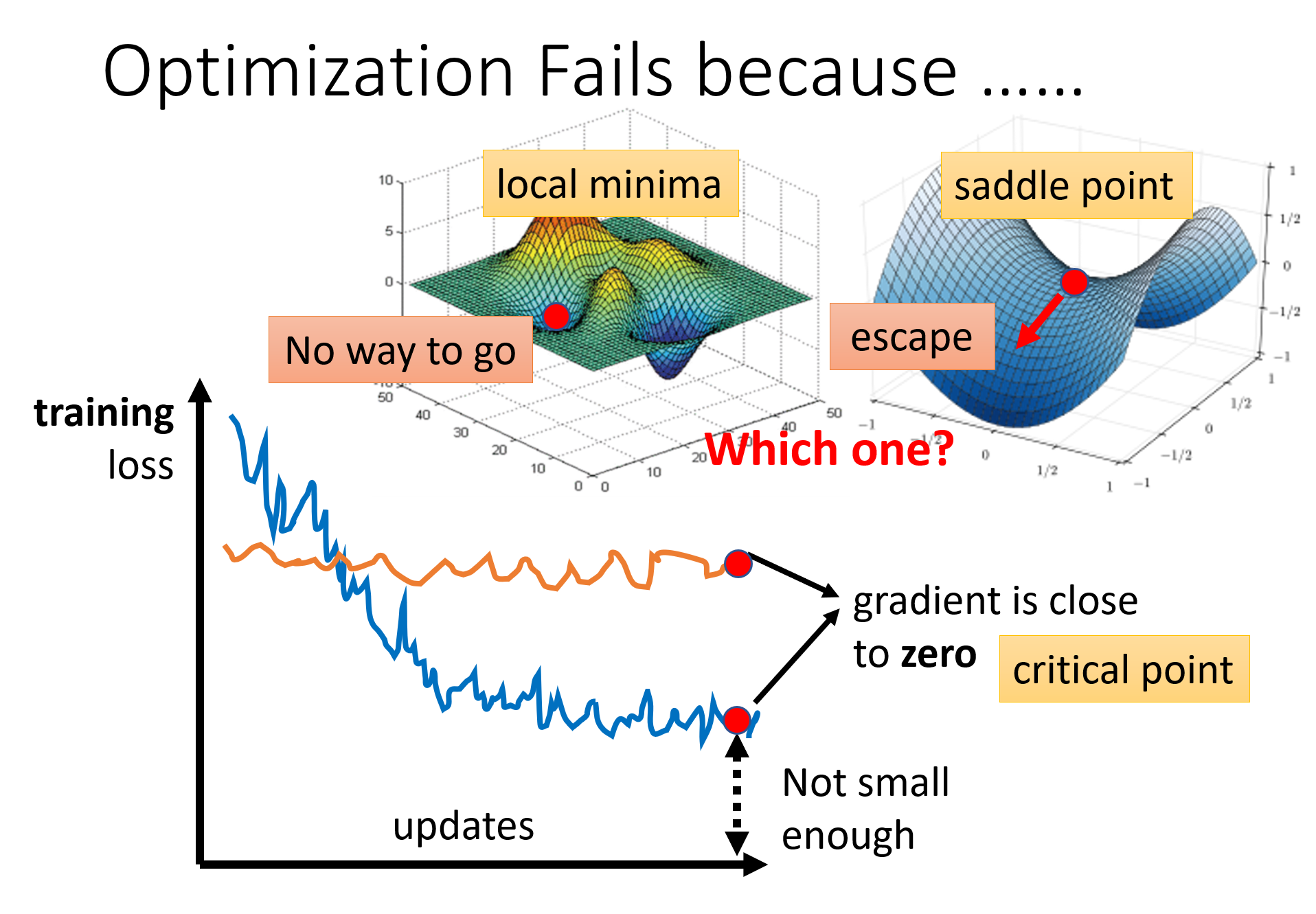
  Gradient is close to zero (training loss did not decrease or is not small enough) caused by meeting critical point (local minima or saddle point)
\[L(\boldsymbol{\theta}) \approx L(\boldsymbol{\theta'}) + (\boldsymbol{\theta} - \boldsymbol{\theta'})^T\boldsymbol{g} + \frac{1}{2} (\boldsymbol{\theta} - \boldsymbol{\theta'})^T H (\boldsymbol{\theta} - \boldsymbol{\theta'})\]
这里的零阶项是损失函数在 $\boldsymbol{\theta'}$ 点的值，一阶项反映的是损失函数在 $\boldsymbol{\theta'}$ 点的线性变化（Gradient/一阶微分），二阶项反映的是损失函数的局部曲率（Hessian/二阶微分）。在 critical point 上，Gradient 项为零，所以要根据 Hessian matrix 来判断。如果二阶项大于零，则在 $\boldsymbol{\theta'}$ 附近有 $L(\boldsymbol{\theta}) > L(\boldsymbol{\theta'})$，即说明 $\boldsymbol{\theta'}$ 点是一个 local minima，计算上只需要算出 Hessian matrix 的 eigenvalue，应有所有的 eigenvalue 都是正的。同理，如果所有的 eigenvalue 都是负的，则为 local maxima。如果 eigenvalue 有正有负，则为 saddle point。

L2 Norm (Euclidean Norm): $\Vert\boldsymbol{x}\Vert_2 = \sqrt{x_1^2 + x_2^2 + \cdots + x_n^2}$

L1 Norm (Manhattan Norm): $\Vert\boldsymbol{x}\Vert_1 = \vert x_1 \vert + \vert x_2 \vert + \cdots + \vert x_n \vert$

L-infinity Norm: $\Vert \boldsymbol{x} \Vert_\infty = \max(\vert x_1 \vert, \vert x_2 \vert, \ldots, \vert x_n \vert)$，常被用来限制向量的最大变化量。在对抗性机器学习中，常用于衡量对抗性扰动的强度，确保这些扰动在每个维度上的最大改变不会超过某个预设的阈值。

计算量大，不会这么做！如果遇到 saddle point，只需要找出负的 eigenvalue（$\lambda < 0$），再找到相对应 $H$ 的 eigenvector $\boldsymbol{u}$，然后得到新的点 $\boldsymbol{\theta} = \boldsymbol{\theta'} + \boldsymbol{u}$，这个点的 loss $L$ 就会更小（$\frac{1}{2} (\boldsymbol{\theta} - \boldsymbol{\theta'})^T H (\boldsymbol{\theta} - \boldsymbol{\theta'}) = \boldsymbol{u}^TH\boldsymbol{u} = \boldsymbol{u}^T(\lambda\boldsymbol{u}) = \lambda\Vert\boldsymbol{u}\Vert_2^2 < 0 \rightarrow L(\boldsymbol{\theta}) < L(\boldsymbol{\theta'})$）。

When you have lots of parameters, perhaps local minima is rare？在低维度看起来是 local minima，但是在更高维度上更有可能是 saddle point，即 local minima 需要满足在各个维度上都是最小（很难做到）。所以当 Training loss 卡在某一个位置时，往往是遇到了 saddle point，而不是 local minima。

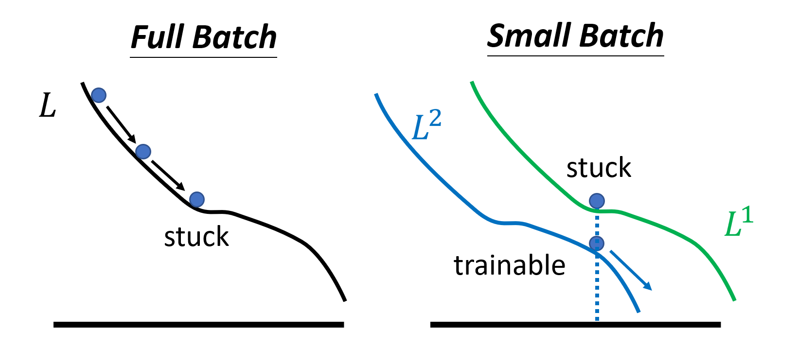
Mini-batch and Momentum can help escape critical points.

Mini-batch

epoch

将 Training data 划分 batch 的时候需要做 shuffle，一个常见的做法是在每个 epoch 开始之前进行划分，使得每一个 epoch 的 batch 都不一样。

在使用 GPU 并行运算的条件下，smaller batch requires longer time for one epoch (seeing all data once)

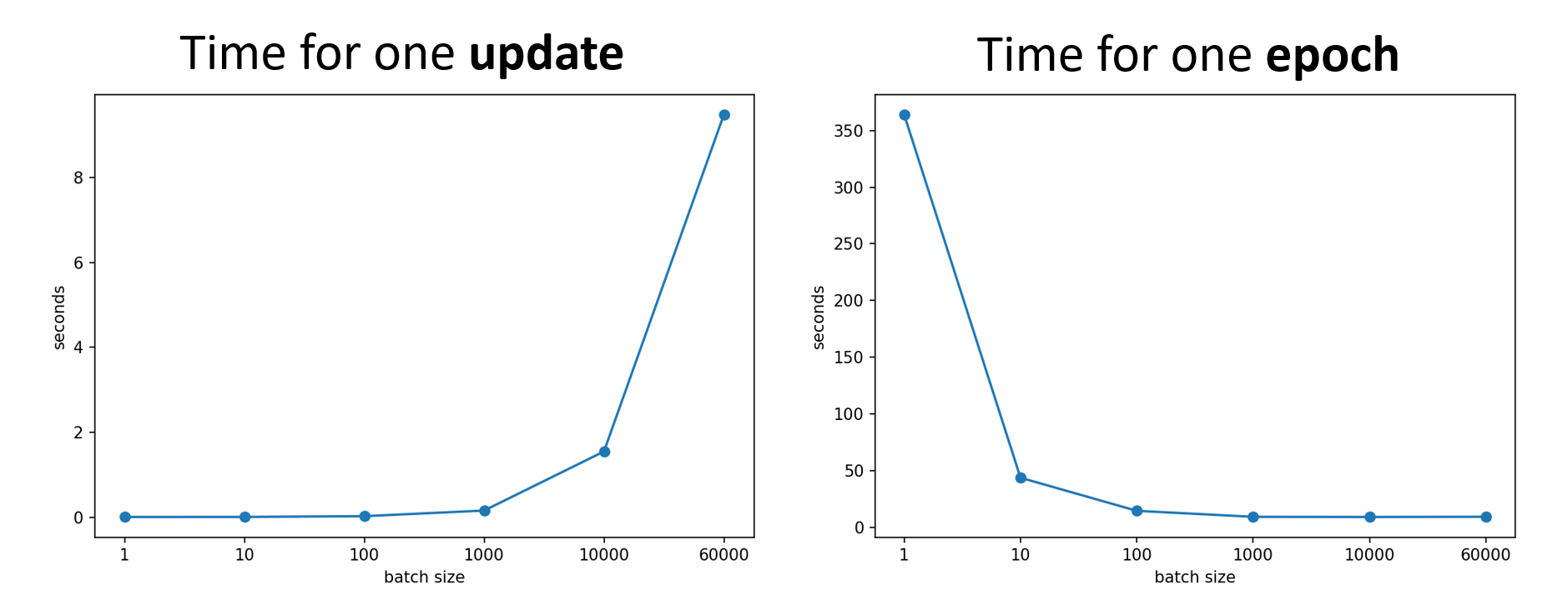
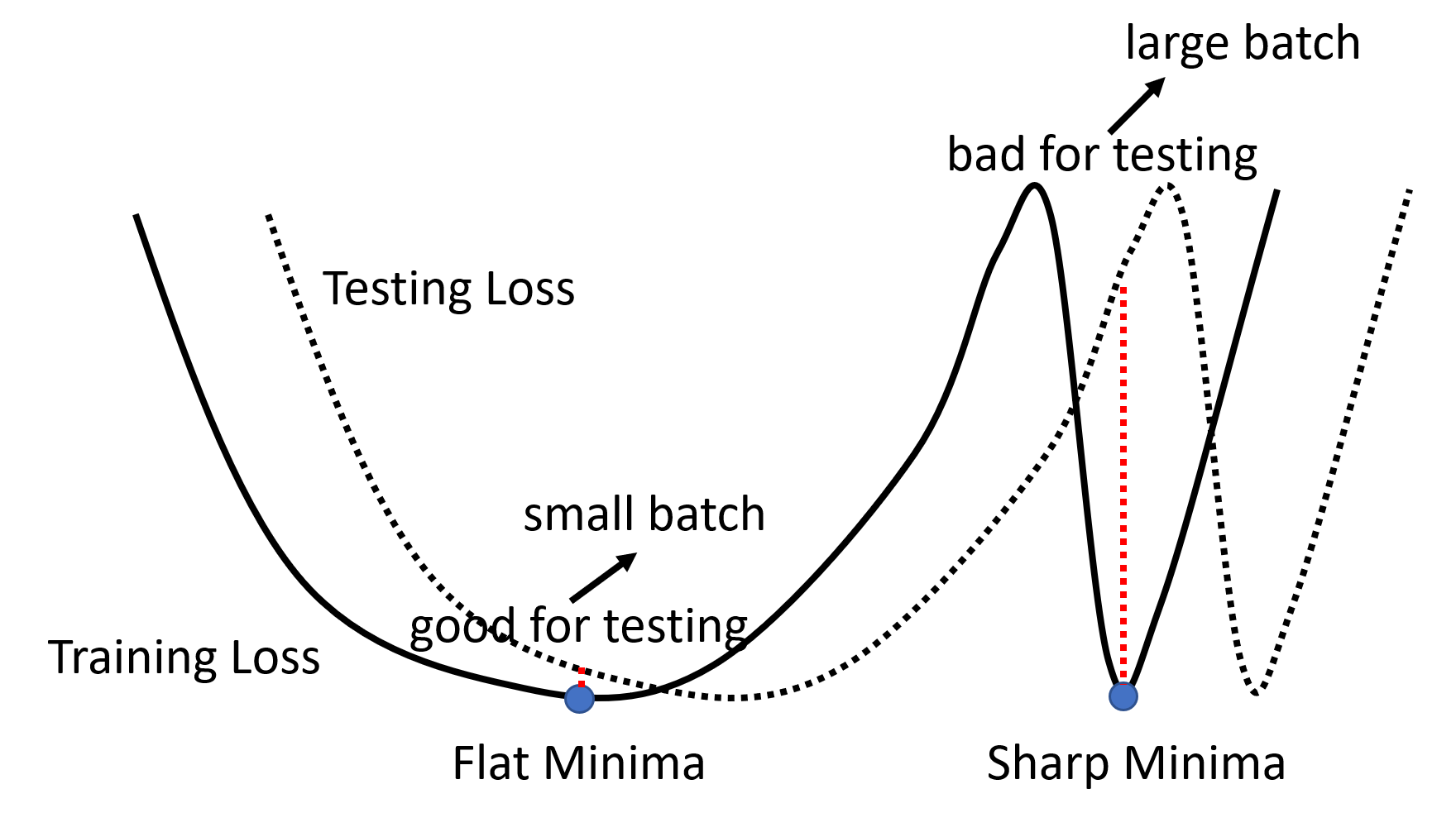
But smaller batch has better performance on training data and testing data (below is one of the explanations)

	Small Batch	Large Batch
Time for one epoch	Slower	Faster
Gradient	Noisy	Stable
Optimization	Better	Worse
Generalization	Better	Worse

总的来说，就是要调整 batch size 这个超参数来做取舍以达到想要的效果（当然也有可能做到鱼与熊掌兼得）。

Momentum

Timestamp - 24:45

Optimization is not just based on gradient, but previous movement (movement is movement of the last step minus gradient at present).

Movement $\boldsymbol{m^i}$ is the weighted sum of all the previous gradient: $\boldsymbol{m^0} = 0, \ \boldsymbol{m^1} = \lambda\boldsymbol{m^0} -\eta\boldsymbol{g^0} = -\eta\boldsymbol{g^0}, \ \boldsymbol{m^2} = \lambda\boldsymbol{m^1} - \eta\boldsymbol{g^1} = -\lambda\eta\boldsymbol{g^0} - \eta\boldsymbol{g^1}$ ($\lambda$ is also a hyperparameter) and parameter $\boldsymbol{\theta}$ updated by

\[\begin{gather*} \boldsymbol{m^i} = \lambda\boldsymbol{m^{i-1}} - \eta\boldsymbol{g^{i-1}} \\ \boldsymbol{\theta^i} = \boldsymbol{\theta^{i-1}} + \boldsymbol{m^i} \end{gather*}\]

因此，参数的更新方向不是完全按照当前 iteration 的 gradient 的方向，而是按照过去所有 gradient 的方向的总和作为更新的方向。

P.S. 这里的 momentum $\boldsymbol{m}$ 写作是 gradient $\boldsymbol{g}$ 的反方向，但是像 Adam 论文中写的是 $\boldsymbol{m}$ 与 $\boldsymbol{g}$ 同方向，所以更新参数 $\boldsymbol{\theta}$ 时要减去 $\boldsymbol{m}$。

Adaptive Learning Rate

Convex error surface (Error Surface describes the relation between loss and parameters) is an ideal situation that has a clear global minima.

训练停滞不一定是由于 critical point (small gradient)，也可能是 learning rate 的原因。

Different parameters needs different learning rate, if gradient is small, learning rate needs to be larger, vice versa.

AdaGrad: Add a parameter dependent parameter $\sigma$ to adjust learning rate in gradient descent formulation. For $i$-th parameter $\boldsymbol{\theta_i^t}$, if gradient is small in $i$-th iteration, then $\sigma_i^t$ is also small, so learning rate will be larger. Hence, learning rate can be adjusted automatically.
\[\begin{gather*} \boldsymbol{\theta_i^{t + 1}} \leftarrow \boldsymbol{\theta_i^t} - \frac{\eta}{\sigma_i^t}\boldsymbol{g_i^t} \\ \sigma_i^t = \sqrt{\frac{1}{t + 1}\sum\limits^t_{i=0}(\boldsymbol{g_i^t})^2} \end{gather*}\]

Root Mean Square (RMS): $\text{RMS} = \sqrt{\frac{1}{n} \sum_{i=1}^{n} x_i^2}$

RMSProp: AdaGrad 默认每一个 gradient 都有同等的重要性（且会记住过去所有的梯度），在此基础上 RMSProp 做出改进在参数 $\sigma_i^t$ 中引入另一个超参数 $\alpha$，从而可以调整当前 iteration 的 gradient 的重要性（选择性地遗忘过去的梯度）。¹
\[\sigma_i^t = \sqrt{\alpha(\sigma_i^{t-1})^2 + (1 - \alpha)(\boldsymbol{g_i^t})^2}, \ 0 < \alpha < 1\]
Adam: RMSProp + Momentum, Momentum decides the direction of update and RMSProp decides the step size of update. And Adam also needs warm up.

Adam Paper 建议使用 PyTorch 预设的参数即可
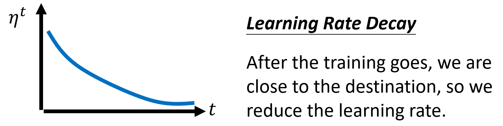
Learning Rate Scheduling: 令学习率随着时间变化，即 $\eta \rightarrow \eta^t$
- Learning Rate Decay
- Warm Up
  
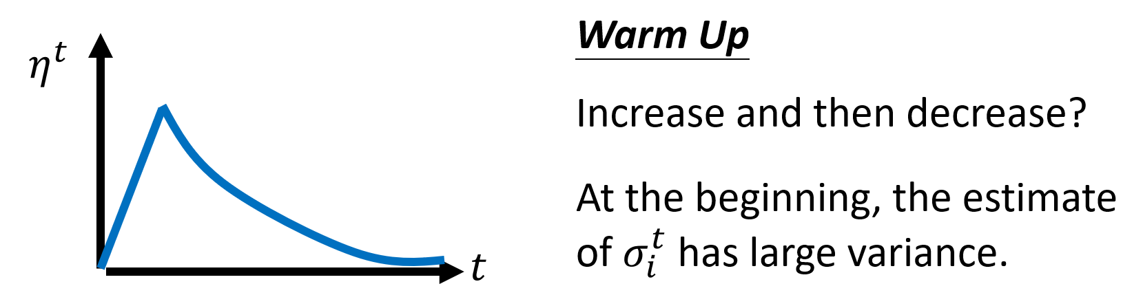
  Warm Up is used in Residual Network, Transformer, BERT, 比较玄学，更多理解见 RAdam
  
  The shape of the curve is like human life, up and down.

Determine it’s caused by model bias or optimization:

Gaining the insights from comparison.
Start from shallower networks (or linear model, SVM, Tree model, etc.), which are easier to optimize.
If deeper networks do not obtain smaller loss on training data, then there is optimization issue.

Training loss is small, testing loss is large
1. Overfitting
  
  Solution:
  - Searching more training data
  - Data augmentation (Creating new data based on the understanding of the problem and the characteristics of data, but need to be reasonable in the real world (like flipping an image horizontally instead of vertically, because the former does not affect the recognition of objects within the image))
  - Constraining model
    - Less parameters, sharing parameters
    - Less features
    - Early stopping
    - Regularization
    - Dropout
2. Mismatch
  
  Training data and test data have different distributions. Be aware of how data is generated.

Trade-off：将 Training set 分为 Training set 和 Validation set，用前者拟合得到模型，根据模型在后者上的结果来选择模型，最后在 Test set 上评估。（尽量）不要用 Test set 上的结果去调整模型。最好的就是直接选择 Validation set 上 loss 最小的模型。P.S. 这里的 Validation set 要具有足够的代表性（保证分布一致）。如果担心单一验证集会过于乐观或代表性不足，也可以用 N-fold Cross-Validation，但这里最后就要用全部的 Training set 来拟合模型。

Classification

为保证分类的各类别之间距离相等（无特定关系），需要用 one-hot vector 来表示类别。

\[\text{softmax} = \frac{\exp(y_i)}{\sum_j\exp(y_j)}\]

通常在分类的最后要加一层 softmax，目的是将输出归一化（各个输出都介于 0 到 1 之间，且它们的和为1），然后再计算输出与 label（one-hot 形式）之间的距离（用 Cross-entropy 来计算 loss）。特别地，当二分类时，用 softmax 和 sigmoid 的效果是一样的。

Posterior Probability（后验概率）：是指在已知某一事件发生的条件下，另一事件发生的概率，它是 Bayes’ Theorem（贝叶斯定理）的核心概念，通常用来在给定观测数据后更新我们对一个假设的可能性的评估，从而为下一步的决策提供依据。此外，后验概率的分布还可以作为不确定性的度量，概率分布如果集中某一类别上则表示模型非常确信其预测，而概率分布如果较为平坦则表示模型对其预测相对不确定。贝叶斯定理的公式：$P(B_i \parallel A) = \frac{P(B_i)P(A \parallel B_i)}{P(A)} = \frac{P(B_i)P(A \parallel B_i)}{\sum^n_{i=1}P(B_i)P(A \parallel B_i)}$。其中，$P(B_i)$ 是 Prior Probability （先验概率），即在没有观测到数据之前认为假设 $B_i$ 为真的概率；$P(B_i \parallel A)$ 是后验概率，即观测到数据 $A$ 出现后认为假设 $B_i$ 为真的概率；$P(A \parallel B_i)$ 是 Likelihood（似然），即在假设 $B_i$ 为真的条件下，观测到数据 $A$ 的概率；$P(A)$ 是数据 $A$ 出现的总概率，保证概率的归一化。

Likelihood 是从果到因考虑问题（给定结果，求导致这个结果的原因的可能性）。

神经网络的原始输出经过 softmax 函数处理后，可以被转换为概率分布，这里每个类别的输出概率可以被解释为在给定输入数据的条件下，该类别为正确类别的后验概率。为什么是后验概率？因为这些概率反映了模型基于当前观测到的数据对每个类别正确性的评估。

Cross-entropy: $e = - \sum_i\hat{y_i} \ln y_i$, minimizing cross-entropy is equivalent to maximizing likelihood.

For classification tasks, cross-entropy is better than MSE (easy to train). In PyTorch, torch.nn.CrossEntropyLoss 自动包含了 softmax 操作，即在使用时会先对模型的输出应用 softmax 函数，再计算交叉熵损失，因此不需要在模型的最后一层手动添加 softmax 激活函数，模型的最后一层输出应直接是未经 softmax 处理的 logits。

因此，改变 loss function 也可以优化 optimization（change the landscape of error surface）。

Optimizers for DL

Optimizers: SGD, SGD with momentum (SGDM), AdaGrad, RMSProp, Adam, AdamW (Hugging Face BERT)

Adam v.s. SGDM

Adam: Fast Training, Large Generalization Gap, Unstable, Possibly Non-convergence, Suitable for NLP, GAN, RL

SGDM: Slow Training, Small Generalization Gap, Stable, Better Convergence, Suitable for CV

Something may help optimization:

Increase Randomness (More Exploration)

Shuffle, Dropout, Gradient Noise
Start from easy

Warm Up, Curriculum Learning, Fine-tuning
Normalization, Regularization

AdamW：在 Adam 中，权重衰减通常是通过在损失函数中加入一个正则项（L2 惩罚）来实现的。在参数更新公式中，这种方式导致权重衰减会受到学习率的影响。而 AdamW 将权重衰减从梯度更新过程中分离出来，允许权重衰减独立于自适应学习率，使其仅依赖于设定的衰减系数，这种方法更接近传统的权重衰减，从而可以提高训练过程的稳定性，并且在一些任务中，如训练深层网络或复杂的模型时，表现得更好。

Tips for DL

DL 其实不容易 Overfitting，像 KNN、Decision Tree 这样的 ML 模型很容易就会在训练集上达到 100% 的 accuracy，这才叫容易 Overfitting。DL 第一个遇到问题最可能是在训练集上根本 train 不起来，accuracy 很低。在训练集上结果好后，再在验证集上评估如果效果差，如果用某些技术解决了 Overfitting 但是发现训练集又变坏了，那就需要再调整让训练集变好，如此反反复复直到在训练集和验证集上表现都足够好。

Activation Function

ReLU：$f(x) = \max(0, x)$ 目前比较常用，其优点为计算速度快且可以解决 vanishing gradient problem。

LeakyReLU：$f(x) = \begin{cases} x & \text{if } x > 0 \\ \alpha x & \text{if } x \le 0 \end{cases}$，$\alpha$ 是一个很小的正数（例如 0.01），有助于避免神经元死亡问题，这使得在训练过程中保持网络的梯度流动。

Early Stopping

如果训练集的 loss 还在下降，但验证集的 loss 反而开始回升，此时应该提前停止训练。

Regularization

Modify the loss function

L2-regularization：$L_{l_2}(\boldsymbol{\theta}) = L(\boldsymbol{\theta}) + \frac{\lambda}{2} \Vert \boldsymbol{\theta} \Vert^2_2$，L2 正则化通过在损失函数中添加一个正则化项来实现，这个正则化项由于是平方项，所以对于较大的参数值会更敏感，从而增大对较大参数值的惩罚（即优化算法会增大参数减小的幅度，以最小化总损失）。因此，L2 正则化能够防止模型过于复杂，有利于防止过拟合。

更新的过程就变为：$\theta \leftarrow \theta - \eta \frac{\partial L_{l2}}{\partial \theta} = \theta - \eta (\frac{\partial L}{\partial \theta} + \lambda \theta) = (1 - \eta \lambda)\theta - \eta \frac{\partial L}{\partial \theta}$，$(1 - \eta \lambda)\theta$ 这一项由于 $\theta$ 会乘上一个很接近于 1 但小于 1 的值，所以会越来越小趋近于 0，因此也被称为 Weight Decay。

Dropout

适用于训练集表现好但验证集表现不好的情况下。

在用每一个 mini-batch 做每一次 update 之前都要重新采样要 dropout 的 neuron，因此每一次 update 用来训练的 network structure 是不同的。Dropout 会让训练的性能变差，但是目标是提升测试（validation）的性能。在测试（validation）时则保留全部的 neuron，需要注意的是，如果训练时 dropout 的比例是 $p\%$，那测试时的所有权重都要乘上 $(1-p)\%$。

Dropout is a kind of ensemble.

3. CNN

Image $\rightarrow$ 3-D tensor (width, height and channel), every pixel of an image is composed of 3 colors (RGB), so 3 channels represent RGB.

Fully Connected Layer: 网络中的每个神经元都与前一层的每一个神经元相连接，在全连接层中，输入的所有特征都会被考虑在内，输入的每个特征都会对每个输出产生影响。全连接层通常用于网络的最后几层，将前面层输出的特征进行汇总和非线性组合，以执行分类、回归或其他任务（数学运算就是矩阵乘法加上偏置项，通常后接一个非线性激活函数）。

Observation 1

只需要对 neuron 输入图像的某一小部分来判断是否具有某些重要的具有代表性的 pattern 即可判断图像中的物体，而不需要每个 neuron 都去看完整的图像。

Same patterns are much smaller than the whole.

Simplification 1

Typical Receptive Field Setting for Simplifying Fully Connected Network

Each receptive field has a set of neurons (e.g., 64, 128).
Stride (e.g., 1, 2) controls the movement step size of the receptive field and it’s best to have overlap between receptive fields.
Padding fills the edges of the image with zeros or other values to control the size of the whole image.

Observation 2

同样的 pattern 可能会出现在不同图像的不同区域，识别同样 pattern 的 neuron 做的事情其实是一样的，只是它们负责的 Receptive Field 有所不同。

The same patterns appear in different regions.

Simplification 2

Parameter Sharing for Different Receptive Fields. Typical setting is that each receptive field has the neurons with the same set of parameters (A set of parameters is called a filter).

Statement 1

Receptive Field + Parameter Sharing = Convolutional Layer (Lower complexity than Fully Connected Layer, and lower risk of overfitting, but larger model bias)

Statement 2

\[\text{Image} \xrightarrow[]{\text{Convolutional Layer}} \text{Feature Map}\]

If convolutional layer has 64 filters, feature map can be seen as “image” with 64 channels (image from 3 channels to 64 channels, i.e., convolution). 每一个卷积层中的 filter 的 channel 数需要等于输入的 image/”image“ 的 channel 数。

Statement 1 and 2 are Same story: The values of filters in statement 2 are the same as parameters (weight and bias) of neurons in statement 1, so when a filter sweeps across the image (i.e., convolution), it’s equal to sharing parameters.

Observation 3

Subsampling the pixels will not change the object $\longrightarrow$ Pooling

Pooling decreases the width and height of the image.

Pooling 在 Convolution 之后使用，并且两者通常交替使用，比如做一次/几次 Convolution 做一次 Pooling。Pooling 主要目的是降低计算量，但是如果识别/侦测的是非常微细的东西，Pooling 所做的 Subsample 可能会对性能有所伤害，要考虑具体应用场景来决定是否要对 network 做 Pooling。

要得到最终的结果，需要对 Pooling 的输出做 Flatten（把矩阵拉直，变成一个向量），再输入到 FC Layer 中，最后再经过 softmax。

Convolutional layer is specifically designed for images, if it’s used for other tasks, need to consider whether these tasks have characteristics similar to images.

But CNN is not invariant to scaling and rotation, so we need data augmentation.

4. Self-attention

Self-attention is to consider the information of the whole sequence

Vector Set as Input and What is the Output

Each vector has an output label
The whole sequence has an output label (e.g., Input molecular graph and output molecular property)
Model decides the number of output labels itself (e.g., Seq2seq)

Dot Product: $\mathbf{A} \cdot \mathbf{B} = a_1b_1 + a_2b_2 + \ldots + a_nb_n = \sum_{i=1}^{n} a_i b_i$

Input of Self-attention can be either input of the whole network or output of a hidden layer

输入向量两两之间相互的关联程度/相似性用 $\alpha$ 来表示，可以通过计算两个向量的点积（点积可以衡量两个向量在各个维度上的值的匹配程度）来得到，点积结果大即关联程度高。

\[\boldsymbol{q^1} = \boldsymbol{a^1}W^q, \ \boldsymbol{k^2} = \boldsymbol{a^2}W^k \longrightarrow \alpha_{1,2} = \boldsymbol{q^1} \boldsymbol{\cdot} \boldsymbol{k^2}\]

如果有四个输入向量 $\boldsymbol{a^i}, \ i=1,2,3,4$，以第一个向量 $\boldsymbol{a^1}$ 为例，会计算出 $\alpha_{1,2}, \ \alpha_{1,3}, \ \alpha_{1,4}$ 以及通常还会有自身与自身的关联程度 $\alpha_{1,1}$，然后通过 softmax（也可为其他的激活函数）得到 $\alpha'$。然后对每一个输入向量乘上一个 $W^v$，再根据 attention scores 来提取信息得到 $\boldsymbol{b^1}$。P.S. $\boldsymbol{b^i}, \ i=1,2,3,4$ 是同时计算出来的，而不是依次。

\[\begin{gather*} \boldsymbol{v^i} = \boldsymbol{a^i}W^v, \ i=1,2,3,4 \\ \boldsymbol{b^j} = \sum\limits_i\alpha'_{j,i}\boldsymbol{v^i}, \ j=1,2,3,4 \end{gather*}\]

值得注意的是，这其中只有 $W^q, W^k, W^v$ 是需要从训练数据中学习的。

P.S. $\boldsymbol{q}$ is query, $\boldsymbol{k}$ is key, $\boldsymbol{v}$ is value, and $\alpha$ is attention score.

Multi-head Self-attention

以 2 heads 和 2 input $\boldsymbol{a^i}, \boldsymbol{a^j}$ 为例，原本 $\boldsymbol{a^i}$ 所对应的 $\boldsymbol{q^i}$ 变成 $\boldsymbol{q^{i,1}}, \boldsymbol{q^{i,2}}$，即 $\boldsymbol{q^{i,1}} = W^{q,1}\boldsymbol{q^i}, \ \boldsymbol{q^{i,2}} = W^{q,2}\boldsymbol{q^i}$，然后在计算输出的时候每一 head 会分开计算。head 1的计算公式为 $\boldsymbol{b^{i,1}} = \text{softmax}(\boldsymbol{q^{i,1}} \boldsymbol{\cdot} \boldsymbol{k^{i,1}})\boldsymbol{v^{i,1}} + \text{softmax}(\boldsymbol{q^{i,1}} \boldsymbol{\cdot} \boldsymbol{k^{j,1}})\boldsymbol{v^{j,1}}$。得到每一 head 的输出后，将这些输出 concatenate $[;]$，然后通过另一个线性变化 $W^O$ 整合不同 head 的信息来得到最终的输出 $\boldsymbol{b^i} = W^O [\boldsymbol{b^{i,1}}; \boldsymbol{b^{i,2}}]$。

Positional Encoding

如果输入的 sequence 的每个元素的位置信息很重要，可以给输入 $\boldsymbol{a^i}$ 添加一个 unique positional vector $\boldsymbol{e^i}$，它可以是 hand-crafted 的，也可以是 learned from data。Paper

Self-attention for a long sequence

If sequence is very long, there need large momery to storage the attention matrix.

Truncated Self-attention

对于 sequence 中的某个/些元素只需要看一定范围内的 attention 即可，而不是看整个 sequence。

Self-attention v.s. CNN

CNN: Self-attention that can only attends in a receptive field (CNN is simplified self-attention)
Self-attention: CNN with learnable receptive field (Self-attention is the complex version of CNN)

CNN is a subset of Self-attention. But more flexible model needs more training data to perform better.

Self-attention v.s. RNN

Timestamp - 35:12 Self-attention is parallel.

Self-attention for Graph

考虑到 edge 的存在，可以不再需要 model 自己学习 node 之间的关联性，只计算有 edge 相连的 node 之间的 attention 即可。相当于 graph 其实就已经是建立在 domain knowledge 之上的。

Self-attention 的缺点是计算量比较大。

5. Transformer

Batch Normalization

Batch Normalization - Training

Batch Normalization can do optimization by changing the landscape of error surface (also the loss function part mentioned above)

如果 feature 的不同 dimension 的 scale 差距很大，就会导致 error surface 在不同方向上的斜率非常不同。如果可以让不同的 dimension 有同样的数值范围，可能就会得到比较好的 error surface，让 training 变得更容易/更快

Feature Normalization: For features $\boldsymbol{x^1}, \boldsymbol{x^2}, \boldsymbol{x^3}, \cdots, \boldsymbol{x^r}, \cdots, \boldsymbol{x^R}$, and for each dimension $i$, the mean is $\mu_i$ and the standard deviation is $\sigma_i$. So the means of all dims are 0, and the stds are 1, $\tilde{\boldsymbol{x}}\boldsymbol{^r_i} \leftarrow \frac{\boldsymbol{x^r_i} - \mu_i}{\sigma_i}$. Feature Normalization can make gradient descent converge faster.

Converge（收敛）：某个过程随着时间的推移逐渐稳定到某个固定值或状态。

当对输入 $\tilde{\boldsymbol{x}}^\boldsymbol{1}$ 做 Feature Normalization 后通过 $W^1$ 得到的 $\boldsymbol{z^1}$ 同样也需要做 Feature Normalization 来保证不同的 dims 有同样的 range，然后再通过激活函数得到这一层的输出 $\boldsymbol{a^1}$。这里的 Feature Normalization 通常是在激活函数之前做，也就是对 $\boldsymbol{z^i}$ 做，即 $\tilde{\boldsymbol{z}}^\boldsymbol{i} \leftarrow \frac{\boldsymbol{z^i} - \boldsymbol{\mu}}{\boldsymbol{\sigma}}$（由于是向量，相减相除都是 element-wise 的）。

$\leftarrow$ 代表赋值（assignment）

由于在训练时通常考虑的是一个 batch，而不是整个 training set，所以也称作 Batch Normalization。

由 $\boldsymbol{z^i}$ 得到的 $\tilde{\boldsymbol{z}}^\boldsymbol{i}$ 的 mean 一定是 0，这会对 network 产生一些限制，可能会有未知的负面影响，所以再加回参数 $\boldsymbol{\gamma}, \boldsymbol{\beta}$ 来让 network 自己学习调整输出的分布，即 $\hat{\boldsymbol{z}}^{\boldsymbol{i}} \leftarrow \boldsymbol{\gamma}\odot\tilde{\boldsymbol{z}}^\boldsymbol{i} + \boldsymbol{\beta}$。通常 $\boldsymbol{\gamma}, \boldsymbol{\beta}$ 的初始值分别为 ones vector 和 zeros vector。

Batch Normalization - Testing

在测试时，由于 Batch Normalization 需要一个 batch 的数据来计算 $\boldsymbol{\mu}$ 和 $\boldsymbol{\sigma}$，但是当用户输入的时候，不可能每次都是恰好一个 batch size 的数据，这时在 PyTorch 中，采用的策略是在训练时每一个 batch 的 $\boldsymbol{\mu}$ 和 $\boldsymbol{\sigma}$ 都会用来算 moving average（假如有 t 个 batch，$\bar{\boldsymbol{\mu}} \leftarrow p\bar{\boldsymbol{\mu}} + (1-p)\boldsymbol{\mu^t}$，$p$ 是超参数，默认为 0.1），然后用 $\bar{\boldsymbol{\mu}}$ 和 $\bar{\boldsymbol{\sigma}}$ 取代 $\boldsymbol{\mu}$ 和 $\boldsymbol{\sigma}$。

Seq2seq

Input a sequence, output a sequence. The output length is determined by model (e.g., speech recognition, machine translation, speech translation, Question Answering

Question Answering (QA) can be done by seq2seq.

\[\begin{gather*} {\large \textbf{Seq2seq Architecture}} \\ \text{Sequence} \longrightarrow \text{Encoder} \longrightarrow \text{Decoder} \longrightarrow \text{Sequence} \end{gather*}\]

Seq2seq’s Encoder

Input vectors, output vectors, i.e., $\boldsymbol{x^1}, \boldsymbol{x^2}, \cdots, \boldsymbol{x^k} \xrightarrow[]{\text{Encoder}} \boldsymbol{h^1}, \boldsymbol{h^2}, \cdots, \boldsymbol{h^k}$

Seq2seq’s Decoder

Autoregressive and Non-autoregressive

内部协变量偏移（Internal Covariate Shift）：训练过程中网络各层的输入分布会随着上一层参数的更新而不断变化，使得网络各层需要不断适应新的输入分布，从而可能导致训练过程缓慢，需要更小的学习率和更细致的参数初始化策略。减少 Internal Covariate Shift 可以加快训练过程，使得模型更快收敛，同时也可以提高模型的训练稳定性，降低梯度爆炸或梯度消失的风险。

Layer Normalization: 独立地对每个样本的所有特征进行归一化，即对 $\begin{bmatrix} x_1 \\ x_2 \\ \vdots \\ x_k \end{bmatrix}$ 求得 mean $\mu$ 和 std $\sigma$，然后通过 $x_i' = \frac{x_i - \mu}{\sigma}$ 计算得到 $\begin{bmatrix} x_1' \\ x_2' \\ \vdots \\ x_k' \end{bmatrix}$，可以减少 Internal Covariate Shift，同时也不像 BN 那样依赖于 batch size，适用于 batch size 较小或需要适应动态 batch size 的情况。

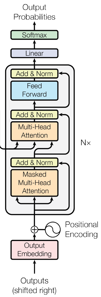
Transformer’s Encoder

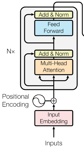
输入需要做 Positional Encoding 后再输入到 Multi-Head Attention (Self-attention) 中；
Self-attention 的每个 output vector 还需要再加上它的 input vector 来当作是新的 output，这样的操作叫做 residual connection；
然后这个新的 output 再去做 Layer Normalization；
Layer Normalization 的输出再输入到 FC Network中，FC Network 在这里也有 residual 的架构；
FC Network 的输出再做一次 Layer Normalization 作为 Transformer’s Encoder 的一个 block 的输出；
Transformer’s Encoder 一共重复 N 次上述的 block。

BOS (begin of sentence)：在 NLP 中，处理文本数据时常常需要明确标示句子的起始和结束位置。BOS 作为一个 token，帮助模型识别句子的开始。这对于训练语言模型、进行序列生成任务（如文本生成、机器翻译等）尤为重要，因为模型需要了解句子结构的边界以更准确地处理和生成文本。同理，EOS (end of sentence) 可以用来表示句子的结束。

token：通常指文本中的一个独立的、有意义的元素，是构成 sentence 的基本单位。在文本处理和分析中，原始文本经常会被分割成 tokens，以便于进一步的处理和分析。

Autoregressive (AR)：基于过去的值来预测未来的值，逐步生成序列的每个元素。在 Autoregressive 模型中，每个时刻的输出不仅依赖于输入变量，还依赖于之前时刻的一个或多个输出。e.g., $X_t = \alpha X_{t-1} + \epsilon_t$

Non-autoregressive (NAR)：一次性地生成整个序列（将整个输入序列一次性送入模型并利用并行计算的能力来同时处理序列中的所有位置），显著提高了生成速度。但是，由于模型可能难以捕捉序列中的长距离依赖关系，所以会牺牲一定的生成质量。

Transformer’s Decoder

Masked Self-attention：举例来说，当产生 $\boldsymbol{b^2}$ 时，只用 $\boldsymbol{q^2}$ 与 $\boldsymbol{k^1}, \boldsymbol{k^2}$ 去计算 attention score，即每个位置只考虑当前和之前的 attention。

Why masked? Consider how does decoder work (i.e., Autoregressive). Decoder 看到的输入是它在前一个时间点自己的输出（初始从 BOS 开始），即 Self-attention 的 $\boldsymbol{a^1}, \boldsymbol{a^2}, \cdots, \boldsymbol{a^i}$ 是 one by one 依次产生的，而不是原来的一次性输入全部。

最后，添加一个 “Stop Token” EOS，当 Decoder 输出 EOS 时整个程序结束，从而使得机器能够自行决定要输出的 sequence 的长度。
Autoregressive Transformer (AT) v.s. Non-autoregressive Transformer (NAT)
- 因为 NAT 是一次性输出整个序列，那么如何决定其输出序列的长度呢？
  1. Another predictor for output length (在 Encoder 后加一个 classifier 来提前给出 Decoder 所输出的序列的长度)
  2. Output a very long sequence, ignoring tokens after EOS
- Advantages: parallel, controllable output length
- Disadvantages: NAT is usually worse than AT
Cross Attention：Encoder 的输出 $\boldsymbol{b^1}, \boldsymbol{b^2}, \cdots, \boldsymbol{b^i}$ 会产生 $\boldsymbol{k^1}, \boldsymbol{k^2}, \cdots, \boldsymbol{k^i}$ 和 $\boldsymbol{v^1}, \boldsymbol{v^2}, \cdots, \boldsymbol{v^i}$，Decoder 通过 Masked Self-attention 输出的向量会产生 Query $\boldsymbol{q}$。$\boldsymbol{q}$ 与 $\boldsymbol{k}$ 点乘得到 $\alpha$，再与 $\boldsymbol{v}$ 加权求和，所得到的向量再输入到 FC Network 中。在 Transformer 中，这里的 $\boldsymbol{k}$ 和 $\boldsymbol{v}$ 来自于 Encoder 的最后一层，$\boldsymbol{q}$ 则来自于 Decoder 的当前层。这样的设置允许 Decoder 的每一层都能够访问到 Encoder 的全部信息。

Transformer’s Training

minimize cross entropy
Teacher Forcing: using the ground truth as decoder’s input. 在早期阶段，可以有效地指导模型学习正确的输出模式，提高效率。但会导致 training 和 inference (testing) 存在一定的 Mismatch。因为在 inference 中，模型必须依赖于自己的输出来生成下一个词，所以模型会看到一些错误的东西，但在 training 中模型看到的始终是正确的。这个现象叫做 Exposure Bias，因此会导致在 inference 中，当模型遇到自己的预测是错误的时会表现不佳，因为它在训练过程中没有足够的机会去学习如何从自己的错误中恢复。Scheduled Sampling 可以通过逐渐地将模型自己的预测引入训练过程中来有效地缓解 Exposure Bias，具体来说，是在训练过程的不同阶段以一定的概率选择使用模型的预测输出而不是真实的上一个输出作为下一个时间步（Time Step）的输入，并且这个概率会随着时间逐渐增加，从而帮助模型在训练过程中逐渐适应其在实际应用中的使用情况。Transformer 并没有用 Scheduled Sampling，要想用的话需要更多的考虑。
Training tips1 - Guided Attention: 引入额外的信息或约束来指导注意力的焦点（或引导注意力的分布，比如让注意力保持从左向右），使模型能够更有效地学习从输入到输出的映射关系。Guided Attention 通常通过在模型的损失函数中加入额外的项来实现，使得模型在训练过程中被鼓励学习符合这些引导的注意力分布，从而在特定任务上达到更好的性能。
Training tips2 - Noise: 当需要机器有创造力时，可以在 Decoder 中加入随机性。在语音合成（Text-to-Speech, TTS）中，模型训练好后需要在测试时添加 Noise 才会让合成出来的声音更像人声（有点违背常理，因为 Noise 通常在训练时添加（e.g., Dropout），让机器看过更多的可能性，从而模型会更 robust）。
Training tips3 - Optimization: When you don’t know how to optimize, just use Reinforcement Learning (RL)! (e.g., loss function is non-differentiable, considering loss function as reward and Decoder as agent)

6. Generation

Network as Generator

The input of the network is not only $\boldsymbol{x}$, but $\boldsymbol{x}$ and a random variable $\boldsymbol{z}$, $\boldsymbol{z}$ is randomly sampled from a distribution, and this distribution is simple enough, i.e., we know its formulation (e.g., Normal/Uniform). So the output of the network $\boldsymbol{y}$ is a complex distribution. And the network here is called generator. The architecture of the generator is totally customizable. P.S. 这些简单的分布选择哪一个差异都不大，只要够简单就行，因为 generator 总是会将其对应到一个复杂的分布。

Especially for the tasks needs “creativity”. Because the same input $\boldsymbol{x}$ can have different outputs $\boldsymbol{y}$.

GAN

GAN 很强大但是局限性在于 unstable training。

本节的讨论都是基于 Unconditional generation: input without $\boldsymbol{x}$

Discriminator is actually a neural network (architecture is customizable) and its output is a scalar (larger means input is real, otherwise, it is fake).

Description

The discriminator’s function is to determine whether the input data is real or fake, the latter being generated by the generator. And the generator’s function is to generate fake data that is as close as possible to the real one. The two are adversarial, making each other stronger and stronger.

Algorithm

Step 1: Randomly Initialize the parameters of generator and discriminator.

For each iteration:

Step 2: Fix generator, and update discriminator. Firstly, sample some vectors from normal distributions (or others) as input to feed into generator, then generator generates some fake objects and we can also sample some real objects from database. Next discriminator learns to assign high scores to the real objects and low scores to the generated objects (Considered as classification or regression).

Step 3: Fix discriminator, and update generator. According to the scores output by discriminator, generator learns how to maximize the scores to the generated objects. 所以这里可以把 discriminator 输出的 score 加一个负号作为 loss，让 loss 越小越好，从而更新 generator 的参数。

Step 4: Repeat step 2 and 3, until both are good enough.

Objective

Divergence（散度）：用于衡量两个概率分布（Probability Distribution）之间的差异或不一致性的程度。例如 KL 散度和 JS 散度都是通过比较两个分布在同一事件集上的概率值来量化分布之间的差异。

KL Divergence (Kullback-Leibler Divergence)：也称为相对熵（Relative Entropy），对于两个概率分布 $P$ 和 $Q$，公式为 $KL(P \parallel Q) = \sum_{x} P(x) \log \frac{P(x)}{Q(x)}$，$x$ 表示每个事件。其中，对数部分用于衡量 $P$ 和 $Q$ 在每个事件上的相对差异，如果 $P(x)$ 和 $Q(x)$ 相等，那么表示两者在该事件上没有差异，则对数部分为 0。$P(x)$ 则是事件 $x$ 在分布 $P$ 中发生的真实概率，如果这个概率很低，那么即使差异很大，它对总的 KL 散度的贡献也会较小。最后两者综合的结果表示从分布 $P$ 到分布 $Q$（分布 $P$ 相对于分布 $Q$）的“信息损失”量，即 KL 散度量化了如果我们假设数据遵循分布 $Q$ 而真实分布为 $P$ 时，我们期望遭受的信息损失。KL 散度越大，意味着使用假设分布 $Q$ 来近似真实分布 $P$ 时会损失更多的信息。局限性：KL 散度是非对称（即 $KL(P \parallel Q) \ne KL(Q \parallel P)$）的且无界的。

JS Divergence (Jensen-Shannon Divergence): 公式为 $JS(P \parallel Q) = \frac{1}{2} KL(P(x) \parallel \frac{P(x) + Q(x)}{2}) + \frac{1}{2} KL(Q(x) \parallel \frac{P(x) + Q(x)}{2})$，相比于 KL 散度，JS 散度是对称且有界（当对数底数为 2 时，范围为 0 到 1）的。当两个概率分布完全相同时，即 $P(x) = Q(x)$ 时，JS 散度为 0。当两个概率分布完全不相交（没有重叠）时，JS 散度达到最大值。可以理解为一个事件在一个分布中发生时（概率大于 0），在另一个分布中一定不发生（概率为 0）。JS 散度可以看作是基于平均分布的比较。JS 散度对于分布中的小变动（如噪声）通常也更加平滑（不敏感）。

Cross Entropy: $H(P, Q) = -\sum_{x} P(x) \log Q(x)$，交叉熵常用作 NN 的损失函数来衡量概率分布 $P$ 和 $Q$ 之间的相似性。交叉熵与 KL 散度之间的关系：$H(P, Q) = H(P) + KL(P \parallel Q)$。因此，交叉熵不仅考虑了当使用分布 $Q$ 来近似分布 $P$ 时的信息损失（分布间差异导致的额外的不确定性），还考虑了分布 $P$ 本身的不确定性。这意味着最小化交叉熵可以间接最小化预测分布与真实分布之间的 KL 散度，从而提高模型的预测准确性。

JS 散度倾向于比较两个分布的相似度，交叉熵倾向于优化一个模型，使其预测分布尽可能接近真实分布。

$P(A \mid B)$ 读作 “P of A given B”

对于 Generator $G$ 和其输出的分布 $P_G$，以及真实数据的分布 $P_{data}$，有

\[G^* = \arg \min\limits_G \text{Div}(P_G, P_{data})\]

The objective is to find a generator $G^*$ that can make minimize the divergence between $P_G$ and $P_{data}$. However, the divergence (e.g., KL or JS) is hard to compute when the distribution is continuous.

Although we do not know how to formulate the continuous distributions $P_G$ and $P_{data}$, we can sample from them.

When it needs to be maximized, it is called an objective function; conversely, it is called a loss function.

Training Discriminator: $D^* = \arg \max\limits_D V(D, G)$ and objective function for discriminator $D$: $V(D, G) = E_{y \sim P_{data}}[\log D(y)] + E_{y \sim P_G}[\log (1-D(y))]$ ($\sim$ represents the random variable $y$ follows the distribution, 遵循/服从于)。因为要最大化 $V$ 的值（最大化 discriminator 区分真假样本的能力），所以希望如果样本是从真实数据中采样的，discriminator 给出的分数越高越好。如果是从 generator 生成的样本中采样的，则分数越小越好。$V(D, G)$ is equal to negative cross entropy, so training discriminator is equal to train classifier, and the maximum objective value $\max\limits_D V(D, G)$ is related to JS divergence (if the two distributions are similar, data sampled from them is mixed, so it’s hard to discriminate and $\max\limits_D V(D, G)$ is small). So we can replace the old objective function $Div(P_G, P_{data})$ with the new one $\max\limits_D V(D, G)$, i.e.,

\[G^* = \arg \min\limits_G \max\limits_D V(D, G)\]

即在给定 generator 的条件下找 discriminator 来 maximize $V(D, G)$，然后再找 generator 来 minimize $\max\limits_D V(D, G)$，具体用 Algorithm 部分的步骤来解。

Tips for GAN

Manifold（流形）：是一个局部具有欧几里得空间（平直空间）性质的高维空间（复杂空间），即存在于高维空间的数据其实可以用潜在的低维流形来表示，或者说在高维空间中实际有效的数据点（即反映数据本质结构和关系的点）可能只占据了一小部分区域，或者说高维空间中的所有点并非都同等重要。流形学习就是学习一种“将数据从高维空间降维到低维空间，还能不损失信息”的映射，从而能够揭示数据的内在结构（非线性 ok），帮助我们更好地表示和理解数据。

JS divergence is not suitable, because $P_G$ and $P_{data}$ are not overlapped

Explanation 1: The nature of data, i.e., both are low-dim manifold in high-dim space, so the overlap can be ignored;

Explanation 2: Even though they have overlap, if sampling is not sufficient, there is always a boundary that can separate them.

Problem: JS divergence is always log2, so even though the distances between two distributions are different, they are same to the JS divergence, which results in the inability to update parameters during training. In this case, binary classifier always achieves 100% accuracy.
WGAN

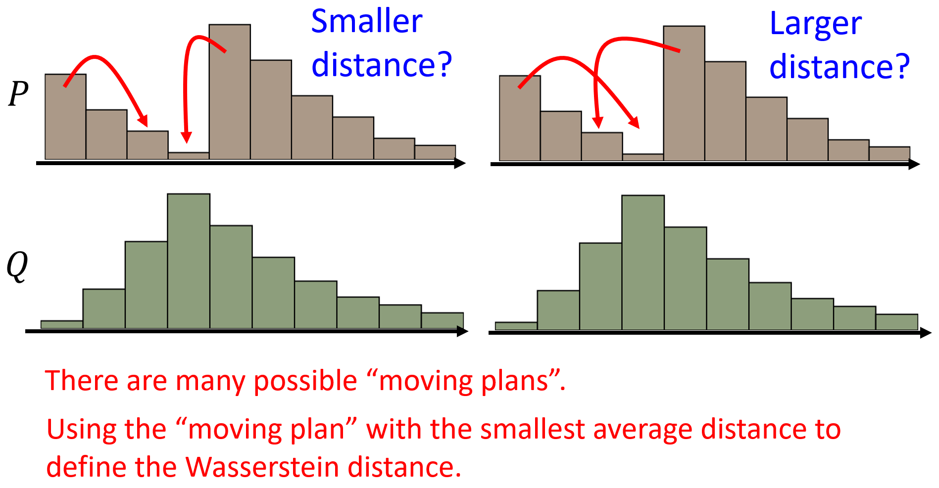
用 Wasserstein distance 替代 JS divergence。Wasserstein distance (Earth Mover’s Distance, EMD) 是指衡量将一个概率分布变换成另一个概率分布所需的最小“成本”或“工作量”。所以如果两个分布没有重叠，当它们之间的距离不同时，Wasserstein distance 也能给出相应不同的值，从而能够进行 optimization，而非像 JS divergence 那样始终是常数。

Lipschitz Continuity：一个函数 $f: X \rightarrow Y$，存在一个实数 $c$，对于该函数定义域 $X$ 上的任意两点 $x_1, x_2$，连接它们的直线的斜率的绝对值不大于这个实数，即 $\frac{\vert f(x_1) - f(x_2) \vert}{\vert x_1 - x_2 \vert} \le c$。它本质上是限制了连续函数斜率的变化，保证了函数的平滑性。1-Lipschitz 即实数 $c$ 的值为 1。

Spectral Normalization：是一种正则化技术，用于约束神经网络中权重矩阵的谱范数（spectral norm），可以控制该层输出相对于输入变化的速度，从而确保神经网络满足 Lipschitz 连续性。Spectral norm 是矩阵的最大奇异值，可以理解为矩阵的最大“拉伸因子”。具体步骤为：1）对于每个权重矩阵 $W$，计算其最大奇异值 $\sigma(W)$；2）对 $W$ 进行归一化，即新的权重矩阵为 $W/\sigma(W)$。其优势在于不需要额外的超参数调整。

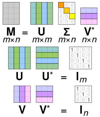
Singular Value Decomposition (SVD，奇异值分解)：给定一个矩阵 $M$，有 $M = U \Sigma V^T$。其中，$U$ 和 $V$ 是 Orthogonal Matrix（如果一个矩阵是正交矩阵，则它和它 transpose 的乘积是 Identity Matrix），$\Sigma$ 是 Diagonal Matrix，对角线上的元素是 $M$ 的奇异值，并且这些奇异值是按照从大到小的顺序排列的。

WGAN 的 optimization 为：
\[D^* = \arg \max\limits_{D \in 1-Lipschitz} \{E_{y \sim P_{data}}[D(y)] - E_{y \sim P_G}[D(y)]\}\]
其中的目标函数的值就当作是 Wasserstein distance。因为目标是前一个 $D(y)$ 要越大越好，后一个则越小越好。所以如果没有 1-Lipschitz 的限制，当真实样本和生成样本没有重叠的时候，discriminator 会分别给出 $\infty$ 和 $-\infty$ 的分数，从而导致 discriminator 的训练无法收敛。并且只要是没有重叠，不论分布之间的距离大小，最后得到的值都会是 $\infty$，这就跟 JS 散度一样了。加上 1-Lipschitz 限制后，因为要求 discriminator 足够平滑，所以当分布之间距离小时，Wasserstein distance 值就会比较小，反之就会比较大，从而保证了训练的稳定性。

WGAN 并没有真正地实现 1-Lipschitz，实际操作上可以用 Spectral Normalization (Keep gradient norm smaller than 1 everywhere) 来实现 1-Lipschitz，也就是 SNGAN。
GAN for Sequence Generation

Gradient 其实是当某一个参数有变化时，对目标造成了多大的影响。当 generator 的参数有一个小变化时，它输出的 distribution 也会有一个小变化，但是这不会影响它最终输出的 token 是哪一个（因为取的是 max），所以 discriminator 输出的分数也不会改变。因此，Gradient descent is not work。
Diversity of GAN

Problem 1: Mode Collapse. 生成器开始生成几乎相同的样本，而无法覆盖到真实数据分布的多样性。

Problem 2: Mode Dropping. 生成器遗漏了一部分真实数据的分布。

检测 diversity 的方法：将 generator 的输出 $y^i$ 输入到一个 classifier 里面，每个 $y^i$ 都会得到一个分布 $P(c \mid y^i)$，将所有的分布取平均，如果平均的分布非常集中（比如都属于某一类），则说明多样性不够。值得注意的是，diversity 是以多个生成器的输出（e.g., 1000 images）来评价的，而 quality 是以单个输出（e.g., 1 image）来评价的。

通过 classifier 的输出的类别可能都是一样的，比如生成的分子不同，但是类别都是化合物；或者生成的人脸不同，但类别都是人脸。所以要用 softmax 之前的 hidden layer 的输出向量，这个向量是不同的，用真实数据和生成数据的这个向量来计算 Frechet Inception Distance，这个值越小多样性越高。

Problem 3: 如何评判 generator 生成的样本是不是 GAN 所 memory 的？Evaluation of GAN is difficult.

Conditional Generation

加回 $\boldsymbol{x}$ ，作为 condition，用来操控 generator 的输出。例如，Text-to-image 的任务，$\boldsymbol{x}$ 就是一段文字，通过 RNN 或 Transformer’s Encoder 等等将其编码为向量再输入到 generator 里。

按照 Unconditional 的训练方法 generator 只需要学习到如何生成真实的数据即可“骗过” discriminator（因为 discriminator 的输入只有 generator 的输出 $\boldsymbol{y}$），并没有学习到所输入的 condition $\boldsymbol{x}$。现在 discriminator 的输入还要包括 $\boldsymbol{x}$，所以 discriminator 的评判标准变为 $\boldsymbol{y}$ is realistic or not + $\boldsymbol{x}$ and $\boldsymbol{y}$ are matched or not。因此，需要成对的输入数据（$\boldsymbol{x}$, $\boldsymbol{y}$ pairs）来训练，实际上，需要给 discriminator 的是完全配对时是 1，$\boldsymbol{y}$ 不够好的时候是 0，还有 $\boldsymbol{y}$ 足够好但是和 $\boldsymbol{x}$ 不匹配也是 0。所以喂给 discriminator 的 pairs 中应该有正确配对的，也应该有错误配对的。

Conditional GAN + Supervised Learning 可以让 generator “骗过” discriminator，同时也让生成的结果最接近“标准答案”（即 condition $\boldsymbol{x}$），例如 pix2pix（按照草稿给出房屋设计图）。特别适用于生成的数据和 condition 的模态一致的情况。

If training data is unpaired, network needs to learn to how to output domain $Y$ from input domain $X$ (e.g., Style Transfer). Similarly, the generator can ignore the input data, but also fools the discriminator. And because the input data is unpaired, so conditional GAN is not work.

Cycle GAN

Add another generator $G_{Y \rightarrow X}$ after the first generator $G_{X \rightarrow Y}$, $G_{Y \rightarrow X}$ is to reconstruct the the output of $G_{X \rightarrow Y}$ from domain $Y$ back to domain $X$. And we hope that the output of $G_{Y \rightarrow X}$ and the input of $G_{X \rightarrow Y}$ are as close as possible, the similarity between them can be considered as equivalent to the distance between two vectors. There is also a discriminator that outputs a scalar to determine whether the output of $G_{X \rightarrow Y}$ belongs to domain $Y$ or not.

The process mentioned above can also be reversed. So Cycle GAN is bidirectional.

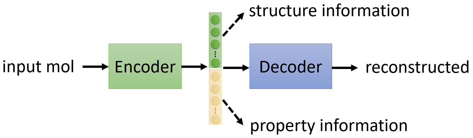
VAE

Auto-Encoder 的流程：

Input data (high-dims) $\longrightarrow$ Encoder $\xrightarrow[]{\text{Compression}}$ vector (low-dims) $\longrightarrow$ Decoder $\xrightarrow[]{\text{Reconstruction}}$ Output data (as close to the input data as possible)

设 Auto-Encoder 的 Encoder 输出的 vector 是 original vector，对于 VAE (Variational Auto-Encoder) 来说，Encoder 输出的是两个 vector $[m_1, m_2, \dots, m_N]$ 和 $[\sigma_1, \sigma_2, \dots, \sigma_N]$（维度和 original vector 一致），然后从一个 normal distribution 中采样一个 vector $[e_1, e_2, \dots, e_N]$，通过 $c_i = \text{exp}(\sigma_i) \times e_i + m_i$ 得到 vector $[c_1, c_2, \dots, c_N]$，这个 vector 是用于输入到 Decoder 中的。并且，训练的过程中不仅要让 output data 和 input data 越接近越好，还需要最小化 $\sum_{i=1}^N(\text{exp}(\sigma_i) - (1 + \sigma_i) + (m_i)^2)$。

这里的 $[m_1, m_2, \dots, m_N]$ 代表了 original vector，$[\sigma_1, \sigma_2, \dots, \sigma_N]$ 代表了 noise 的 variance，从而决定了 noise 的大小（因为 $[e_1, e_2, \dots, e_N]$ 的 variance 是固定的），取 exponential 保证 variance 一定是正的。因此，$[c_1, c_2, \dots, c_N]$ 相当于 original vector with noise。这个 variance 的大小应该是多少是机器在训练时自己学出来的，但是如果不加限制，variance 一定会倾向于为 0，因此给它一个限制让 variance 不能太小 $\sum_{i=1}^N(\text{exp}(\sigma_i) - (1 + \sigma_i) + (m_i)^2)$，式中 $\text{exp}(\sigma_i) - (1 + \sigma_i)$ 的最低点为 $\sigma_i = 0$ 时，所以 $\text{exp}(\sigma_i)$ 的 variance 最小值为 1。$(m_i)^2$ 这一项则相当于做 L2 regularization。

我们想要的是 estimate the probability distribution

Multinomial Distribution：用于描述在具有多个可能结果的实验中，每个结果出现次数的概率，属于一种离散概率分布。其 PMF (Probability Mass Function) 为 $P(X_1 = x_1, X_2 = x_2, \dots, X_k = x_k) = \frac{n!}{x_1! x_2! \cdots x_k!} p_1^{x_1} p_2^{x_2} \cdots p_k^{x_k}$，并且有 $\sum^k_{i=1}p_i=1$，$\sum^k_{i=1}x_i=n$。

Gaussian Mixture Model：由若干个高斯分布组成，每个高斯分布在混合中都有自己的比重，每个数据点都被看作是由这些高斯分布中的一个生成的。其公式为 $P(x) = \sum_m P(m)P(x \mid m)$，$m \sim P(m)$ 表示从一个 multinomial distribution 中采样出第 $m$ 个高斯分布，$x$ 是从 $m$ 中采样得到的，即 $x \mid m \sim N(\mu^m, \sigma^m)$。

Maximum Likelihood Estimation：用于从一组给定的数据中估计模型的参数，核心思想是选择可以使观测到的数据出现概率（即似然）最大的参数值作为最佳估计。首先，假设有数据集 $D$，包含 $n$ 个独立同分布的观测数据点 $\{x_1, x_2, \dots, x_n\}$ 和模型参数 $\theta$。定义似然函数 $L(\theta)$ 为在参数 $\theta$ 下观察到数据集 $D$ 的概率 $L(\theta) = P(D \mid \theta) = \prod^n_{i=1} P(x_i \mid \theta)$。然后取对数将乘积转换为求和 $\log L(\theta) = \sum^n_{i=1} \log P(x_i \mid \theta)$，然后对对数似然函数求导并令其为 0 $\frac{d}{d\theta} \log L(\theta) = 0$，即可求出使对数似然函数最大化的参数值。

$P(z,x) = P(z \mid x)P(x)$，$P(z,x)$ 是 $z$ 和 $x$ 同时发生的联合概率。

上述是 VAE 的直观解释，数学解释如下：

基于 Gaussian Mixture Model 的原理，首先从 normal distribution 中 sample 出一个 vector $z$。$z$ 的每一个维度代表了一个属性（attribute）。从 $z$ 中采样可以对应到不同的 normal distribution，所以由 $z$ 可以决定 normal distribution $P(x \mid z)$ 的 mean 和 variance，即 $\mu(z)$ 和 $\sigma(z)$，写作 $x \mid z \sim N(\mu(z), \sigma(z))$。由于 $z$ 是 continuous 的，所以 $\mu(z)$ 和 $\sigma(z)$ 有无限多的可能，可以用 NN 来学（$z$ 为输入，$\mu(z)$ 和 $\sigma(z)$ 为输出）。从而得到 $P(x) = \int\limits_{z}P(z)P(x \mid z)dz$，$P(z)$ 也是一个 normal distribution。这里要解决的是 $\mu(z)$ 和 $\sigma(z)$ 需要被估计，它的 criterion 是 maximize the likelihood $L = \sum\limits_x \log P(x)$ of the observed $x$，即需要调整 NN 的参数使得 $L$ 最大。另外，还需要一个分布 $Q(z \mid x)$ with $z \mid x \sim N(\mu'(x), \sigma'(x))$ 来决定 $P(z)$ 的 mean 和 variance，即 $\mu'(x)$ 和 $\sigma'(x)$。所以需要另一个 NN’，输入 $x$ 输出 $\mu'(x)$ 和 $\sigma'(x)$。因此，NN（$P(x \mid z)$）就相当于 VAE 的 Decoder，NN’（$Q(z \mid x)$）就相当于 VAE 的 Encoder。

针对 criterion 进行推导：

$$ \begin{align*} \log P(x) &= \int\limits_z Q(z \mid x) \log P(x) dz \ , \ (Q(z \mid x) \text{ can be any distribution, so the integral = 1}) \\ &= \int\limits_z Q(z \mid x) \log (\frac{P(z,x)}{P(z \mid x)})dz \\ &= \int\limits_z Q(z \mid x) \log (\frac{P(z,x)}{Q(z \mid x)} \frac{Q(z \mid x)}{P(z \mid x)}) \\ &= \int\limits_z Q(z \mid x) \log (\frac{P(z,x)}{Q(z \mid x)})dz + \int\limits_z Q(z \mid x) \log (\frac{Q(z \mid x)}{P(z \mid x)})dz \\ &= \int\limits_z Q(z \mid x) \log (\frac{P(x \mid z)P(z)}{Q(z \mid x)})dz + \int\limits_z Q(z \mid x) \log (\frac{Q(z \mid x)}{P(z \mid x)})dz \ , \ (\text{the first term is lower bound} \ L_b \ , \ \text{the second term is KL divergence which is} \ge 0) \\ &= L_b + KL(Q(z \mid x) \parallel P(z \mid x)) \end{align*} $$

对于 lower bound $L_b = \int\limits_z Q(z \mid x) \log (\frac{P(x \mid z)P(z)}{Q(z \mid x)})dz$，未知的是 $P(x \mid z)$ 和 $Q(z \mid x)$。原本依据 $P(x) = \int\limits_{z}P(z)P(x \mid z)dz$ 我们只需要找 $P(x \mid z)$ 来最大化 likelihood，现在则需要找 $P(x \mid z)$ 和 $Q(z \mid x)$ 来最大化 $L_b$。如果还是只找 $P(x \mid z)$ 来最大化 $L_b$，则有可能 $L_b$ 增加但 likelihood 反而减小，因为不知道它们之间的差距是多少，likelihood 减小也会比 $L_b$ 大。因为 $\log P(x)$ 的大小与 $Q(z \mid x)$ 无关，所以如果先固定住 $P(x \mid z)$（即 $\log P(x)$ 的大小保持不变）再调 $Q(z \mid x)$ 去最大化 $L_b$，就可以让 $L_b$ 越来越接近 likelihood（$\log P(x)$）。等到两者相等时，再增大 $L_b$ 就可以保证 likelihood 一定也是增大的（因为 $\log P(x) \ge L_b$）。但是总归来说 VAE 直接优化的是 $L_b$，而不是 likelihood，所以这两者之间具体的差距到底是多少我们并不清楚，这也是 VAE 的局限性。

\[\begin{align*} L_b &= \int\limits_z Q(z \mid x) \log (\frac{P(x \mid z)P(z)}{Q(z \mid x)})dz \\ &= \int\limits_z Q(z \mid x) \log (\frac{P(z)}{Q(z \mid x)})dz + \int\limits_z Q(z \mid x) \log P(x \mid z)dz \\ &= -KL(Q(z \mid x) \parallel P(z)) + \int\limits_z Q(z \mid x) \log P(x \mid z)dz \end{align*}\]

对于 $L_b$ 的第一项 $-KL(Q(z \mid x) \parallel P(z))$，最小化的方法是调 $Q(z \mid x)$ 所对应的 NN’ 的参数让它产生的 distribution 和一个 normal distribution 越接近越好。最小化第一项，其实就是最小化 $\sum_{i=1}^N(\text{exp}(\sigma_i) - (1 + \sigma_i) + (m_i)^2)$。

对于 $L_b$ 的第二项 $\int\limits_z Q(z \mid x) \log P(x \mid z)dz$，可以想成是用 $Q(z \mid x)$ 对 $\log P(x \mid z)$ 做 weighted sum，所以就可以看作是一个期望值 $\int\limits_z Q(z \mid x) \log P(x \mid z)dz = E_{Q(z \mid x)}[\log P(x \mid z)]$。相当于向 NN’ 输入一个 $x$，从 NN’ 输出的一个 distribution（$Q(z \mid x)$）中可以采样出一个 $z$，然后需要最大化由这个 $z$ 再产生 $x$ 的概率（$\log P(x \mid z)$），要做到最大化需要将 $z$ 输入到 NN 中，NN 会输出 $\mu(x)$ 和 $\sigma(x)$，希望 $\mu(x)$ 和 $x$ 越接近越好（在 normal distribution 中 $\mu(x)$ 这个点的概率是最高的）。

因此，$L_b$ 就是 VAE 的 loss function。

VAE 的问题：VAE 可能只是会模仿，而没有办法创新。

Flow-based Model

Flow-based model can directly optimize the objective function $G^* = \arg \max\limits_G \sum^n_{i=1} \log P_G(x^i)$, i.e., maximizing the likelihood, instead of indirectly minimizing the divergence $G^* = \arg \min\limits_G \text{Div}(P_G, P_{data})$.

Jacobian Matrix：如果有一个函数 $\boldsymbol{x} = f(\boldsymbol{z})$，其中向量 $\boldsymbol{x}$ 是关于向量 $\boldsymbol{z}$ 的函数，Jacobian Matrix 可以表示为 $\boldsymbol{x}$ 关于 $\boldsymbol{z}$ 的所有一阶偏导数。如果 $\boldsymbol{x}$ 由 $m$ 个分量组成，$\boldsymbol{z}$ 由 $n$ 个分量组成，则 Jacobian Matrix $\boldsymbol{J}$ 为：
\[\boldsymbol{J}_f = \begin{bmatrix} \frac{\partial x_1}{\partial z_1} & \frac{\partial x_1}{\partial z_2} & \cdots & \frac{\partial x_1}{\partial z_n} \\ \frac{\partial x_2}{\partial z_1} & \frac{\partial x_2}{\partial z_2} & \cdots & \frac{\partial x_2}{\partial z_n} \\ \vdots & \vdots & \ddots & \vdots \\ \frac{\partial x_m}{\partial z_1} & \frac{\partial x_m}{\partial z_2} & \cdots & \frac{\partial x_m}{\partial z_n} \end{bmatrix}\]
可以把 $f$ 当作 generator，$\boldsymbol{z}$ 当作 input，$\boldsymbol{x}$ 当作 output (generation)。

如果有一个 $f$ 的反函数 $\boldsymbol{z} = f^{-1}(\boldsymbol{x})$，其 Jacobian Matrix $\boldsymbol{J}_{f^{-1}}$ 与 $\boldsymbol{J}_f$ 相乘的结果为单位矩阵，即 $\boldsymbol{J}_f \boldsymbol{J}_{f^{-1}} = I$。

Determinant：The determinant of a square matrix is a scalar that provides information about the matrix. 因为有 $\det(A) \cdot \det(A^{-1}) = 1$，所以有 $\det(\boldsymbol{J}_f) \cdot \det(\boldsymbol{J}_{f^{-1}}) = 1$。二阶行列式的几何意义是二维空间中平行四边形的面积，三阶行列式的几何意义是三维空间中平行六面体的体积，更高阶行列式的几何意义是高维空间中的“体积”。另外，一个矩阵做 transpose 不会改变它的 determinant，即 $\det(A) = \det(A^T)$。

Change of Variable Theorem：假设有一个分布 ${\pi(\boldsymbol{z})}$（相当于 generator 输入的分布）和一个函数 $\boldsymbol{x} = f(\boldsymbol{z})$，$\boldsymbol{x}$ 也形成一个分布为 $p(\boldsymbol{x})$（相当于 generator 输出的分布），在分布 ${\pi(\boldsymbol{z})}$ 上有一点 $z'$，它的 probability density value 是 $\pi(z')$，$z'$ 通过函数后会得到 $x'$，它的 probability density value 是 $p(x')$。$\pi(z')$ 与 $p(x')$ 之间存在关系：$p(x')\vert\det(\boldsymbol{J}_f)\vert = \pi(z')$ 等同于 $p(x') = \pi(z')\vert\det(\boldsymbol{J}_{f^{-1}})\vert$。

由 Change of Variable Theorem，可以将 $G^* = \arg \max\limits_G \sum^n_{i=1} \log p_G(x^i)$ 中的 $\log p_G(x^i)$ 表示出来，即 $p_G(x^i) = \pi(z^i)\vert\det(\boldsymbol{J}_{G^{-1}})\vert$ 和 $z^i = G^{-1}(x^i)$，进一步推导有 $\log p_G(x^i) = \log \pi(G^{-1}(x^i)) + \log \vert\det(\boldsymbol{J}_{G^{-1}})\vert$。但是算 $\log p_G(x^i)$ 的这个式子要有两个前提，一是需要计算 $\boldsymbol{J}_{G^{-1}}$，即计算 $\boldsymbol{J}_G$，尽管只需要知道怎么计算 $\frac{\partial{x_i}}{\partial{z_i}}$ 即可，但是 $\boldsymbol{J}_G$ 可能会很大，导致计算 $\det(\boldsymbol{J}_G)$ 的运算量非常大。二是 $G^{-1}$ 是可被计算的，所以要求 $G$ 必须是 invertible 的，则输入 $\boldsymbol{z}$ 的维度和输出 $\boldsymbol{x}$ 的维度就需要保持一致。因此，Flow-based Model 的 $G$ 具有一定的限制性。

既然如此，那就将多个 $G$ 依次连接起来（所以叫 Flow），对于 $\{G_1, \dots, G_N\}$，有 $p_K(x^i) = \pi(z^i)(\vert\det(\boldsymbol{J}_{G^{-1}_1})\vert) \cdots (\vert\det(\boldsymbol{J}_{G^{-1}_N})\vert)$，

所以有 $\log p_N(x^i) = \log \pi(z^i) + \sum\limits^N_{n=1} \log \vert\det(\boldsymbol{J}_{G^{-1}_N})\vert$ 和 $z^i = G^{-1}_1(\cdots G^{-1}_N(x^i))$。

虽然用于生成的是 $G$，但实际训练的是 $G^{-1}$，即从 $p_{data}(x)$ 中采样 $x^i$，然后输入进 $G^{-1}$ 得到 $z^i = G^{-1}(x^i)$。对于 $\log p_G(x^i) = \log \pi(G^{-1}(x^i)) + \log \vert\det(\boldsymbol{J}_{G^{-1}})\vert$ 的第一项 $\log \pi(z^i)$，因为 $\pi$ 是一个 normal distribution，所以 $z^i$ 为 zero vector 时，$\pi(z^i)$ 最大。但是如果经过训练后 $z^i$ 都是 zero vector，会导致 $\boldsymbol{J}_{G^{-1}}$ 为 zero matrix，$\det(\boldsymbol{J}_{G^{-1}}) = 0$，则第二项会趋近于 $-\infty$，从而导致无法最大化 $\log p_G(x^i)$。所以最大化时要同时考虑这两项，第一项让 $z^i$ 趋近于 zero vector，第二项限制不会让所有的 $z^i$ 都变为 zero vector。

Flow-based model 中常用的 $G$ 是 Coupling Layer，它被用于 RealNVP 和 Glow 中。Coupling Layer 的核心思想是将输入分割成两部分，然后以一种方式修改其中一部分，并且这种修改依赖于另一部分的值，同时保持另一部分不变。Coupling Layer 允许进行复杂的变换，同时可以保持整个变换过程的可逆性。

对于一个 $D$ 维的输入向量 $z_D$，将其分成两部分 $(z_1, \dots, z_d)$ 和 $(z_{d+1}, \dots, z_D)$，前一部分保持不变输出 $(x_1, \dots, x_d)$，并且前一部分分别通过函数 $F$ 和函数 $H$ 得到 $(\beta_{d+1}, \dots, \beta_D)$ 和 $(\gamma_{d+1}, \dots, \gamma_D)$（$F$ 和 $H$ 是任意的），然后通过 $x_{i > d} = \beta_{i > d} \cdot z_{i > d} + \gamma_{i > d}$ 计算得到 $(x_{d+1}, \dots, x_D)$。可逆性体现在，当我们知道 $(x_1, \dots, x_d)$ 和 $(x_{d+1}, \dots, x_D)$ 时，对于前者，由于不变可以直接通过 $z_{i \le d} = x_{i \le d}$ 得到 $(z_1, \dots, z_d)$。然后将其正向通过 $F$ 和 $H$ 可以分别得到 $(\beta_{d+1}, \dots, \beta_D)$ 和 $(\gamma_{d+1}, \dots, \gamma_D)$，就可以根据公式 $z_{i > d} = \frac{x_{i>d} - \gamma_{i>d}}{\beta_{i>d}}$ 得到 $(z_{d+1}, \dots, z_D)$。因此，依据可逆性就可以算出 $z^i$。

对于 $\det(\boldsymbol{J}_G)$ 的计算，具体看视频 Timestamp - 49:28，最后公式为 $\det(\boldsymbol{J}_G) = \beta_{d+1}\beta_{d+2} \cdots \beta_D$，因此也很容易计算。

在对 Coupling Layer 进行堆叠（stack）时，需要在某些位置换一下不变的那一部分的位置，可以防止最初设定的不变的那一部分最后的输出还是和输入（随机采样的 noise）一样。

在 GLOW 中还用了一种方法 1x1 Convolution，给定一个 3x3 的 Matrix $W$（3 channels）作为 $G$，通过学习这个 $W$ 做到 shuffle the channels。$W$ 也需要是 invertible 的。

Diffusion Model

生成分子的多样性：VAE、FLOW-based Model

生成分子的质量和细节：GAN、Diffusion Model

7. Self-Supervised Learning

Self-Supervised Learning 是通过利用输入的无标记数据本身的结构来生成标签（一部分数据作为输入，另一部分则作为这个输入的预期输出或标签），进而训练模型，从而无需依赖外部的、成本高昂的标注过程。这种学习方法允许模型通过预测任务来自我学习，从而提取和理解数据的内在结构和特征。

BERT (Encoder-Only)

BERT (Bidirectional Encoder Representations from Transformers) is an Encoder.

Masking Input

Randomly masking some tokens, with the method of masking also chosen randomly: there’re 2 methods, one is to use a special token (e.g., [MASK]), and the other is to use another random token.

然后将 masked token 通过 BERT，其输出做一个 Linear 的 transform 和 softmax 后得到一个分布，再将这个分布与 ground truth 计算 cross-entropy。训练 BERT 使其能够成功预测 masked token 是什么（填空题），相当于一个分类问题。

Masking Input 任务就是一个自监督学习的过程，这个过程不需要外部的标签，因为正确的标签（即被 masked 之前的 token）已经包含在输入中。

Next Sentence Prediction

Add a [CLS] token at the beginning, and add a [SEP] token between two sentences. BERT 处理整个序列，为序列中的每个 token 输出一个向量，但是只有 [CLS] 的向量随后被输入到一个线性层中（这个向量能够捕获整个输入序列的上下文信息（Self-attention）/ 看过整个 sentence 了），根据最终输出的 class 来预测第二个句子是否为第一个句子的逻辑后续。

But NSP is maybe not useful. 所以有以下几种改进：

RoBERTa: Robustly Optimized BERT Approach;
ALBERT: Sentence Order Prediction (SOP).

Fine-tune

BERT 可以通过 fine-tune（need a little bit labeled data）后用于各种 downstream tasks，相当于干细胞。在 fine-tune 中，向模型中输入少量有标记的数据，模型的所有参数（包括 BERT 的原始参数和线性层的新参数）通常都会根据特定任务的损失函数进行优化，以最小化预测输出和实际标签之间的差异，从而提高模型在该任务上的表现。

Pre-train

在 fine-tune 之前产生 BERT 的过程是 Self-Supervised Learning，也叫做 Pre-train。

The use of BERT: Pre-train + Fine-tune can be considered as Semi-supervised Learning (i.e., A large amount of unlabeled data and a small amount of labeled data).

Case 1: Input is sequence, output is class. Add a [CLS] token before the sequence, BERT outputs a vector for each token fed into it, but only the output vector of [CLS] will be input into Linear, and finally output the class. BERT and Linear both need to update parameters, the parameters of Linear is random initialization, but BERT is initiated by Pre-train.

Case 2: Input is sequence, output is also sequence, and both have the same length. BERT outputs a vector for each token fed into it, each vector will be input into Linear, and get its output class.

Case 3: Input is two sequences, output is class. Add a [CLS] token at the beginning, and add a [SEP] token between two sequences. The rest as in case 1.

Case 4: QA。对 BERT 输入一个 sequence，得到 sequence 中每个 token 对应的输出向量 $\boldsymbol{t^i}$，随机初始化一个向量 $\boldsymbol{v}$，将这两者做 Self-attention 后通过 softmax 输出每个 token 对应的概率，最后输出概率最高的 token。也可以初始化两个向量，可以输出由两个 token 组成的这个 sequence 的范围。上述基于正确答案一定在输入的 sequence 里面。

In general，最常见的用法是：BERT 是预训练好的，后面接一个 Linear Classifier，再通过少量的有标记的数据微调两者的参数即可。

BERT 只是 Pre-train 了一个 Encoder，那么如何 Pre-train 一个 seq2seq model 呢？需要将 input sequence 弄坏（corrupted），然后希望 Decoder 输出的 sequence 和弄坏前一模一样（Encoder 和 Decoder 由 cross attention 连接）。弄坏的方法：Mask token、Delete token、打乱顺序、或 Mask + 打乱等等。BART

Cosine Similarity：对于 n 维向量 $\boldsymbol{A}$ 和 $\boldsymbol{B}$，它们的余弦相似度为
\[\text{cosine similarity} = \cos(\theta) = \frac{\boldsymbol{A} \cdot \boldsymbol{B}}{\Vert \boldsymbol{A} \Vert \Vert \boldsymbol{B} \Vert} = \frac{\sum\limits_{i=1}^{n} A_i B_i}{\sqrt{\sum\limits_{i=1}^{n} A_i^2} \sqrt{\sum\limits_{i=1}^{n} B_i^2}}\]
余弦相似度可以很好地衡量两个向量方向的一致性，而忽略它们的大小。

Sequence 的 token 经过 BERT 处理后输出的向量可以称之为 embedding。同样的 token 在不同的上下文中可能代表的意思就不同，所以它们的 embedding 也会不同，计算 embedding 之间的余弦相似度可以用于判断其相似性。BERT 在学习做填空题的过程中（Masking input）也许就是学习从上下文（context）中获取信息来进行预测，由于这里的 embedding 是考虑了上下文信息的，所以可以称之为 contextual embedding。

GPT (Decoder-Only)

GPT (Generative Pre-trained Transformer) 的任务是预测下一个出现的 token 是什么，所以 GPT 具有生成的能力。首先输入 <BOS> token，GPT 输出相应的 embedding，embedding 会通过 Linear Transform 输出一个分布，然后优化其与真实分布之间的交叉熵，以此类推。相当于 Transformer 的 Decoder，只不过 GPT 是经过预训练的且没有 Cross Attention 那部分，只有 Masked Self-attention 那部分。

Prompt：指输入给模型的文本片段，模型据此生成相应的输出，即 Prompt 用于指导模型的生成。

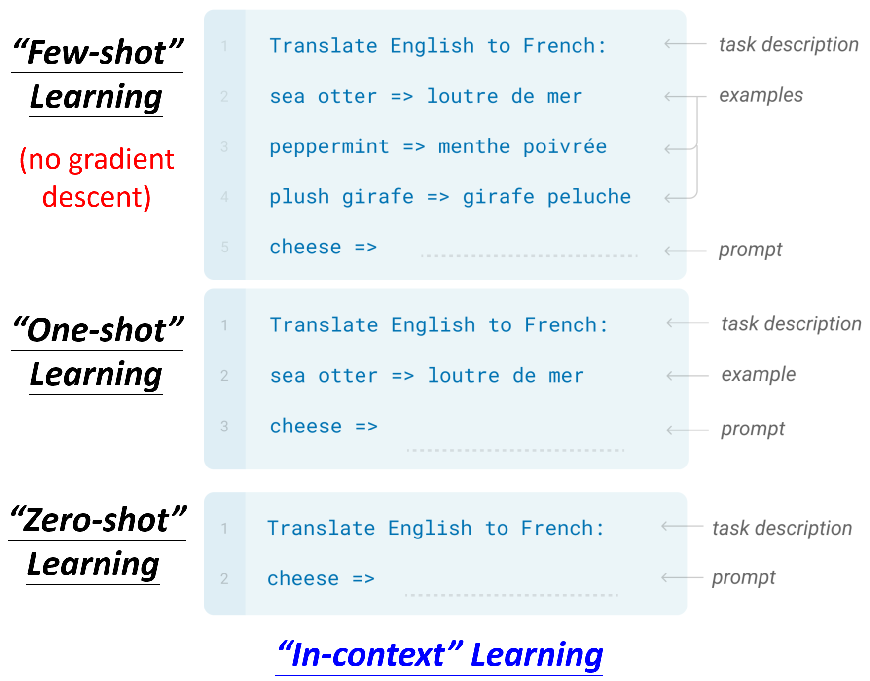
The use of GPT in downstream tasks: Description, example, and prompt.

GPT 基于大规模的预训练和理解上下文的能力，能够在仅有少量所提供的样本的情况下快速适应新的任务，并生成与这些样本相似的输出。这使得 GPT 在很多情况下能够实现或接近专门针对特定任务进行微调的效果。

在 GPT 中的 Few-shot / One-shot / Zero-shot Learning，和一般的不一样，这里并没有做 gradient descent，也就没有微调 GPT 的参数。所以在文献中称作 In-context Learning。

GPT-3 Paper Video

Auto-encoder

Here, vector can be called embedding, representation or feature. And this vector is usually used for downstream tasks.

Auto-encoder 中间输出低维向量的层又被称作 Bottleneck，Bottleneck 强制 Auto-encoder 在有限的维度中捕获输入数据的最重要特征，以便在 Decoder 中尽可能准确地重建输入。因此，Auto-encoder也可以用来做 Dimension Reduction。

虽然输入数据的维度很高，从表面上看比较复杂，但是实际的变化可能是有限的，所以可以用更简单的方法来表示它。那么在下游的任务中，可能只需要比较少的训练数据就可以让模型学到本来应该学到的东西。

De-noising Auto-encoder

给原本的输入加上 noise 作为 Encoder 新的输入，但是 Decoder 重建的还是没有 noise 的输入。BERT 的 Mask Input 其实也相当于是加上 noise。

Feature Disentanglement

Feature Disentanglement 的目的是尝试搞清楚 encoder 输出的 embedding 中，各个/些维度分别代表了什么实际的含义。

Discrete Latent Representation

原本 encoder 输出的 embedding 中的值是 continuous 的，现在使用离散值来表示隐含的特征或状态，每个隐含状态可以对应到一组有限的标签或类别上，从而使得模型可以更简洁地捕捉到关键的信息。比如可以是 Binary（每一维代表某个特征有或没有）或者 One-hot，或者设定一个 codebook（ a set of vectors），计算 embedding 与这些向量之间的相似度，然后将其中相似度最大的向量再输入到 decoder 中，这里的 codebook 也是需要从训练数据中学习的。

In general，embedding 从原来的无限种可能变成了有限种可能。

VAE 则是 encoder 将输入数据映射到一个 latent space（通常是多维正态分布），而非直接映射到一个固定的 latent vector，decoder 再从该分布中 sample 来生成数据，这样 VAE 不仅能够重建输入样本，还能够生成新的数据样本。

Auto-encoder 可以应用于 Anomaly Detection（异常检测），比如 Cancer Detection，难点在于负样本通常很少，所以一般的分类很难 work。

Recent Advances

TODO

Generative Approach

Predictive Approach

Contrastive Learning

Bootstrapping Approach

8. Explainable AI (XAI)

模型可解释性库：Captum - Model Interpretability for PyTorch

目前的 DL：

未来的目标：根据解释的结果来修正模型

Explainable：给予黑箱可解释的能力

Interpretable：解释的对象本来就不是黑箱

Goal of XAI

We do not need to completely know how an ML model works. Because we do not completely know how human brains work, but we trust the decisions of humans!

Why we trust the decisions of humans? Usually, You need a reason (or an excuse) to convince people to believe you (The Copy Machine Study by Ellen Langer). So Good XAI make people (your customers, your boss, yourself) acceptable/comfortable/happy.

我们不知道机器到底真正在想什么，我们希望的是通过某些方法解读出来的东西是人看起来会觉得很开心的（然后就可以编故事说机器就是这么想的）。

Local Explanation & Global Explanation

给定一个 classifier，以及其 input (e.g., molecule) 和 output (e.g., non-toxic)。Local Explanation 问的是“为什么这个分子没有毒性”；Global Explanation 问的是“什么样的分子是没有毒性的”，而不是针对某个特定的分子。

Local Explanation: Explain the Decision

Which component of input data is critical?

从 gradient 的角度，对于 $\{x_1, \cdots, x_n, \cdots, x_N\} \longrightarrow \{x_1, \cdots, x_n +\Delta x, \cdots, x_N\}$，有 $e \longrightarrow \Delta e$，这里的每一个 $x$ 是一个 component，举例来说，对应 image 而言就是一个 pixel，对于 sequence 而言就是一个 token。$e$ 就是 loss。如果某个 $x$ 加上很小的 $\Delta x$，$\Delta e$ 却很大，则说明这个 component 是重要的。因此，可以用 $\vert\frac{\Delta e}{\Delta x}\vert$ 来代表 $x_n$ 的重要性，实际上就是把 $x_n$ 对 loss 做偏微分。把所有的这个比值都算出来后，就可以得到 Saliency Map。

SmoothGrad: Randomly add noises to the input, get saliency maps of the noisy input, and average them. 可以更明显地展示出 saliency map 中对模型决策重要的区域。

只考虑 gradient 会有 gradient saturation 的限制，可以采用 Integrated gradient 来替代。
How a network processes the input data?
- Visualization - 可视化观察网络某个层的输出。
- Probing - 训练一个探针（其实就是一个分类器）插入到网络的某一层中，将这一层输出的 embeddings 输入到分类器中，通过分类器的输出判断目前的 embeddings 到哪一个阶段了或是否学到了什么。但是要注意分类器是否训练成功，因为如果 accuracy 很低，有可能是机器没有学到，也有可能是机器学到了但是分类器训练得很烂，或者是 accuracy 很高，可能因为机器没有学好但是分类器过拟合导致乐观估计。

Global Explanation: Explain the Whole Model

首先 Training a generator with data: input low-dim vector $z$ into a generator $G$ (GAN, VAE, etc.) and the generator outputs $X$ ($X = G(z)$)。然后将 $X$ 输入到一个 classifier 中输出 $y$，希望找到一个 $z$ 使得 $y$ 中的某一个 dim / 某一个类别的概率越高越好，即 $z^* = \arg \max\limits_z y_i$，最后将 $z^*$ 输入到 $G$ 中，观察产生的 $X^*$ 是什么样子，从而可以知道在机器眼中某一个类别是长什么样子的。

还可以尝试用简单的 Linear Model 尽可能地模仿复杂黑盒模型的行为，然后再去分析 Linear Model 也许就可以解释复杂模型。例如 LIME (Local Interpretable Model-Agnostic Explanations) 是用 Linear Model 去模仿复杂模型的一小个区域内的行为，因为 Linear Model 能力有限，很难模仿整个复杂模型的行为。LIME Video1, LIME Video2

9. Adversarial Attack

对于药物设计来说，目前研究的重点更倾向于提高模型的预测准确性和可靠性或解决特定的生物医学问题，而不是对抗潜在的对抗性攻击（安全性）。另外，药物设计领域要构造有效的对抗性样本也比较困难。

10. Domain Adaptation

Domain adaptation can be considered a part of transfer learning.

Domain shift: Training and testing data have different distributons.

Source domain 是 with labeled data 的，随着对 target domain 的了解程度不同，有不同的 domain adaptation 的方法。

在 target domain 上有大量数据且有标签：

直接做训练就好了，根本不需要做 domain adaptation。
在 target domain 上有少量数据且有标签：

用这些少量数据来对已经在 source domain 上训练好的模型进行微调，需要注意的是，由于数据量很少，所以不要在 target domain 上跑太多的 epoch（maybe 个位数？），避免过拟合。
在 target domain 上有大量数据但无标签：

Basic Idea：训练两个 Feature Extractor，分别接收来自 source domain 和 target domain 的输入，然后输出各自的 feature（一个 vector）。Feature Extractor 被训练成能够抽取出两者共同的部分，即各自的 feature 的分布几乎相同。

Domain Adversarial Training

可以将一个 classifier 视为 feature extractor 和 label predictor 两部分，其中哪些部分算 feature extractor，哪些部分算 label predictor 是自行决定的（也算是一个 hyperparameter）。然后再训练一个二元的 domain classifier，它的输入是 feature extractor 所输出的 feature，输出是判断这个 feature 来自于哪个 domain。domain classifier 要做的事是能够正确分类原本来自于哪个 domain，而 feature extractor 则是要模糊界限骗过 domain classifier。所以可以看作是 feature extractor 扮演 generator 的角色，domain classifier 扮演 discriminator 的角色。

以数学公式的角度来看，对于 label predictor，存在参数 $\boldsymbol{\theta_p}$ 和 loss $L$，要求得 $\boldsymbol{\theta_p^*} = \arg \min\limits_{\boldsymbol{\theta_p}}L$；对于 domain classifier，存在参数 $\boldsymbol{\theta_d}$ 和 loss $L_d$，要求得 $\boldsymbol{\theta_d^*} = \arg \min\limits_{\boldsymbol{\theta_d}}L_d$；对于 feature extractor，存在参数 $\boldsymbol{\theta_f}$，要求得 $\boldsymbol{\theta_f^*} = \arg \min\limits_{\boldsymbol{\theta_f}}L - L_d$。

以上是假设两个 domain 内类别集完全相同的情况，但实际上这可能并不总是成立，Universal Domain Adaptation 考虑了 target domain 可能包含 source domain 未见过的新类别，同时也可能缺少 source domain 中的一些类别。目标是使模型能够识别和适应 target domain 中的已知类别（即两者共有的类别），同时对于 target domain 特有的未知类别，模型也能够进行有效的区分和处理。

在 target domain 上有少量数据且无标签：

Testing Time Training (TTT)
对 target domain 一无所知：

Domain Generalization

11. Deep RL

在有标签的数据收集有困难且不知道正确答案的情况下可以考虑 RL。

Machine Learning ≈ Looking for a Function

在 RL 中会有一个 Actor (or Agent) 和一个 Environment，两者会进行互动，Environment 会给 Actor 一个 Observation (or State) 作为其输入，Actor 看到这个 Observation 后会输出一个 Action 去影响 Environment，Environment 改变后就会产生新的 Observation，再进行下一次的互动。所以，Actor 在这里其实就是我们要找的 Function（$\text{Action} = f(\text{Observation})$）。同时，在互动的过程中，Environment 会不断地给 Actor 一些 Reward 来告诉它现在的 Action 是好的还是不好的。最终 Function 的目标是要最大化所获得的 Reward 的总和。

RL Framework (Also 3 Steps)

Function with Unknown

This function is “Actor”, usually called “Policy Network”. The input of policy network is the observation of machine represented as a vector or a matrix. The output is the score for each possible action. The architecture of network is customized. The usual strategy for selecting which action to take is randomly sampling based on the scores as the corresponding probabilities. RL 的结果受 Sample 的影响非常大。
Define Loss Function from Training Data

完成一次 Game Over（达到目标状态/完成任务/任务失败）的整个过程，称作是一个 episode，并得到一个 Total Reward（或者称作 Return）$R = \sum^T_{t=1}r_t$，目标就是要在一个 episode 或多个 episode 中最大化累积的奖励 $R$ ，也可以说 $-R$ 就是 loss。
Optimization

存在一个互动过程 $\begin{gather*} env \rightarrow s_0 \rightarrow actor \rightarrow a_0 \rightarrow env \rightarrow s_1 \rightarrow actor \\ \rightarrow a_1 \rightarrow env \rightarrow s_2 \rightarrow actor \rightarrow a_2 \rightarrow \cdots \end{gather*}$，可以用 trajectory（轨迹）来描述，即 $\tau = (s_0, a_0, s_1, a_1, s_2, a_2, \cdots)$。同时，在这个互动过程中的每个时间步 $t$，reward $r_t$ 的获得都需要依据 $s_t$ 和 $a_t$，所以有 $R(\tau) = \sum^T_{t=1}r_t$。因此，Optimization 的做法就是调 Network（Actor）的参数使 $R(\tau)$ 的数值越大越好。

难点在于：1）Actor 的输出是有随机性的，因为 $a_1$ 是 randomly sample 产生的。给定一个 $s_1$，每次输出的 $a_1$ 不一定一样。（用期望值）2）Environment 和 Reward 都是 black box，很难解释它们的输出是为什么。（只需要与环境交互，不需要了解环境的内部机制）3）Environment 和 Reward 往往也是有随机性的。（用期望值）

对于 Actor 来说，有 $s \longrightarrow \text{Actor}(\text{with param} \ \boldsymbol{\theta}) \longrightarrow a$，如果在特定的 $s$ 的情况下想要输出特定的 $a$，可以计算 $a$ 与 ground truth $\hat{a}$ 之间的交叉熵 $e$。假设有一组训练数据对 $\{s_1, \hat{a}_1\}, \{s_2, \hat{a}_2\}, \{s_3, \hat{a}_3\}, \cdots, \{s_N, \hat{a}_N\}$，如果期待 Actor 能够执行的行为是 take action $\hat{a}_1, \hat{a}_3$ 且 don’t take action $\hat{a}_2$，则 loss 为 $L = e_1 - e_2 + e_3 \cdots$，然后再去 learn 参数 $\boldsymbol{\theta}$ 使 loss 最小（$\boldsymbol{\theta}^* = \arg \min\limits_{\boldsymbol{\theta}}L$）。更进一步，如果每个行为并不是只有好或不好，而是有一个程度可以衡量（不再是一个 binary 的问题），即每一训练数据对 $\{s_t, \hat{a}_t\}$ 都有相对应的一个分数 $A_t$ 作为想要执行该行为的程度。因此，loss 也就变为 $L = \sum A_t e_t$。

那么现在的问题是应该如何正确地获得训练数据对 $\{s_t, \hat{a}_t\}$ 和分数 $A_t$？

Version 0：首先随机初始化一个 Actor，在与 Environment 的交互中得到训练数据对 $\{s_t, a_t\}$，然后在多个 episode 中收集到足够的数据。Reward $r_t$ 就当作 action 的分数 $A_t$（$A_t = r_t$）。但是，由于一个 action 不仅会影响当前的 reward，还会影响后续的 observation，进而影响后续的 reward。所以 Version 0 是一个 short-sighted version。

Reward Delay: Actor has to sacrifice immediate reward (or do something that cannot get any reward) to gain more long-term reward.

Version 1：改进了 Version 0 不合理的点，将以当前点来看未来所有的 reward 加起来来评估当前 action 的好坏，即计算 cumulative reward $G_t = r_t + r_{t+1} + \cdots + r_N = \sum^N_{n=t}r_n$，令 $A_t = G_t$。这样即使当前的 reward 为 0，只看当前的 reward 无法判断 action 的好坏，但是由于 action 还会造成后续的一系列影响，所以也能够知道当前的 action 是好还是坏。

Version 2：由于 $G_t$ 的公式是加和后续所有的 $r$，可能有 $r_t$ 对距离很远的 $r$ 的贡献很小。所以进一步改进了 $G_t$ 的公式，设定一个 discount factor $\gamma < 1$，从而有 Discounted Cumulative Reward $G_t' = r_t + \gamma r_{t+1} + \gamma^2 r_{t+2} + \cdots + \gamma^{N-t} r_N = \sum^N_{n=t} \gamma^{n-t} r_n$，令 $A_t = G_t'$。

Version 3：由于 reward 好还是坏是相对的，所以需要做 Normalization（也能够降低方差）。可以让所有的 $G_t'$ 都减去一个 baseline $b$（$A_t = G_t' - b$）来实现。

Policy Gradient

alt=”Youtube Video”

Initialize actor network parameters $\boldsymbol{\theta^0}$
For training iteration $i$ = $1$ to $T$:
- Using actor $\boldsymbol{\theta^{i-1}}$ to interact with the environment
- Obtain data $\{s_1, a_1\}, \{s_2, a_2\}, \{s_3, a_3\}, \cdots, \{s_N, a_N\}$ (Data collection is in the “for loop” of training iterations)
- Compute $A_1, A_2, \cdots, A_N$
- Compute loss $L$
- Update parameters $\boldsymbol{\theta^i} \leftarrow \boldsymbol{\theta^{i-1}} - \eta \nabla L$

Each time you update the model parameters, you need to collect the whole training set again. One explanation is that the data collected by $\boldsymbol{\theta^{i-1}}$ is the result of $\boldsymbol{\theta^{i-1}}$ interacting with the environment, so that is the experience of $\boldsymbol{\theta^{i-1}}$. This experience can be used to update $\boldsymbol{\theta^{i-1}}$, however, maybe not be good for $\boldsymbol{\theta^{i}}$. (The same action results in different rewards for actors with different capabilities)

另一种讲法（衔接 PPO）：

在给定 Actor 的参数 $\theta$ 下，与环境互动得到某一个 trajectory $\tau$ 的概率为 $p_{\theta}(\tau) = p(s_1) \prod\limits^T_{t=1} p_{\theta}(a_t \mid s_t) p(s_{t+1} \mid s_t,a_t)$，所以 Reward $R(\tau) = \sum\limits^T_{t=1} r_t$ 在这里应该是 Expected Reward $\bar{R_{\theta}} = \sum\limits_{\tau} R(\tau) p_{\theta}(\tau) = E_{\tau \sim p_{\theta}(\tau)}[R(\tau)]$。因此可以计算出 gradient 为

$$ \begin{align*} \nabla \bar{R_{\theta}} = \sum\limits_{\tau} R(\tau) \nabla p_{\theta}(\tau) &= \sum\limits_{\tau} R(\tau) p_{\theta}(\tau) \frac{\nabla p_{\theta}(\tau)}{p_{\theta}(\tau)} \\ &= \sum\limits_{\tau} R(\tau) p_{\theta}(\tau) \nabla \log p_{\theta}(\tau) \ , \ (\text{可以推广到 } \nabla f(x) = f(x) \nabla \log f(x)) \\ &= E_{\tau \sim p_{\theta}(\tau)}[R(\tau) \nabla \log p_{\theta}(\tau)] \\ &\approx \frac{1}{N} \sum\limits^N_{n=1} R(\tau^n) \nabla \log p_{\theta}(\tau^n) \\ &= \frac{1}{N} \sum\limits^N_{n=1} \sum\limits^{T_n}_{t=1} R(\tau^n) \nabla \log p_{\theta}(a^n_t \mid s^n_t) \ , \ (\text{对于 } p_{\theta}(\tau^n) \text{ 只有 } p_{\theta}(a_t \mid s_t) \text{ 这一项与 } \theta \text{ 有关}) \end{align*} $$

可以直观理解为如果在某个 $s_t$ 执行的 $a_t$ 导致 $R(\tau)$ 是正的（大于 baseline 更合理），就增加 $\{s_t, a_t\}$ 这一项的概率；反之，则减少概率。

所以，就可以用 gradient ascent 来做 update（每一次 update 前都需要先收集 $\tau^n$ 和 $R(\tau^n)$），即 $\theta \leftarrow \theta + \eta \nabla \bar{R_{\theta}}$。

Cross-Entropy Loss 的公式为：$L(\theta) = - \frac{1}{N} \sum\limits^N_{i=1} \sum\limits^C_{j=1} y_{ij} \log(p(y=j \mid x_i;\theta))$，其中 $C$ 指有 $C$ 个类别，$y_{ij}$ 是一个指示变量，如果样本 $i$ 属于类别 $j$，则其值为 1，否则为 0。对于单个样本 $x_i$，$p(y=j \mid x_i;\theta)$ 为模型对每个类别 $j$ 的预测概率。

Log-Likelihood 的公式为：$\log L(\theta) = \sum\limits^N_{i=1} \sum\limits^C_{j=1} y_{ij} \log(p(y=j \mid x_i;\theta))$

因此，对于分类问题，我们在最小化交叉熵损失时，实际上是在最大化对数似然，所以最小化交叉熵等同于最大化似然（交叉熵直接衡量了模型预测概率分布与真实概率分布之间的差异，而最大化对数似然意味着寻找能够使得模型预测概率最接近真实标签概率的模型参数）。

具体操作上，对于 Actor 输出 $a_t$（选择采取哪一个动作）可以看作是一个分类问题（输出给定状态下动作的概率分布），由于最小化交叉熵等同于最大化似然，所以最大化 $\frac{1}{N} \sum\limits^N_{n=1} \sum\limits^{T_n}_{t=1} \log p_{\theta}(a^n_t \mid s^n_t)$ 这个目标函数就可以通过最小化交叉熵损失来实现，而它的梯度 $\frac{1}{N} \sum\limits^N_{n=1} \sum\limits^{T_n}_{t=1} \nabla \log p_{\theta}(a^n_t \mid s^n_t)$ 在 PyTorch 中可以自动计算。在这个基础上，只需要在损失函数前乘上一个 weight，即 $R(\tau^n)$。

另外，考虑 baseline 的话，Expected Reward 的 gradient 就变为 $\nabla \bar{R_{\theta}} = \frac{1}{N} \sum\limits^N_{n=1} \sum\limits^{T_n}_{t=1} (R(\tau^n) - b) \nabla \log p_{\theta}(a^n_t \mid s^n_t)$，$b$ 可以取 $E[R(\tau)]$，$E[R(\tau)]$ 是会随着 training 不断改变的，即每得到一个 $R(\tau^n)$，其值就会更新。

对于一个 $\tau$ 中的所有 action 都赋予相同的权重（$R(\tau^n)-b$）看似并不合理，一个做法是用 $\sum\limits^{T_n}_{t=t'} r^n_{t'}$ 替换 $R(\tau^n) = \sum\limits^{T_n}_{t=1} r^n_t$，防止在这个 action 发生之前的 reward 的影响，认为只有在这个 action 发生之后的所有 reward 是与它有关的。更进一步，加一个 discount factor $\gamma < 1$ 减小离 $t'$ 较远的 reward 的影响（action 对远端的 reward 的贡献会逐渐减小），即 $\sum\limits^{T_n}_{t=t'} r^n_{t'}$ 变为 $\sum\limits^{T_n}_{t=t'} \gamma^{t-t'} r^n_{t'}$。因此，可以说 total reward 是 state-dependent。$(\sum\limits^{T_n}_{t=t'} \gamma^{t-t'} r^n_{t'} - b)$ 这一项也被称为 Advantage Function，用 $A^{\theta}(s_t,a_t)$ 来表示。

Mentioned above is “On-policy”, i.e., the actor to train and the actor to interact is the same.

“Off-policy” is that the two can be different. In this way, we do not have to collect data after each update, it enables the use of previously collected data. But the actor to train has to know its difference from the actor to interact. The most commonly used technique is Proximal Policy Optimization (PPO).

Exploration：Actor 在收集数据时的随机性需要大一点，才能收集到更丰富的数据（尝试更多的 Action），因为如果有些 Action 从来没有被执行过，那根本就无法知道这个 Action 好或不好。可能的做法是：1）增大 Actor 输出的策略分布的 entropy（即概率分布更均匀），从而增大随机性（降低预测性）；2）在 Actor 的参数上加 noise。

PPO

Importance Sampling

For $E_{x \sim p}[f(x)] \approx \frac{1}{N} \sum^N_{i=1} f(x^i)$, $x^i$ is sampled from distribution $p(x)$. But if we only have $x^i$ sampled from distribution $q(x)$, the formula is modified to $E_{x \sim p}[f(x)] = \int f(x)p(x)dx = \int f(x)\frac{p(x)}{q(x)}q(x)dx = E_{x \sim q}[f(x)\frac{p(x)}{q(x)}]$，可以理解为因为变成了从 $q(x)$ 中 sample data，所以对 sample 出来的每一笔 data 都需要乘上一个 weight $\frac{p(x)}{q(x)}$ 来修正这两个分布之间的差异。实作上，这两个分布之间的差异不宜过大，如果它们之间差异过大，会导致它们的 variance 差很多，此时 sample 的次数不够多就会导致它们的 expectation 相同无法成立。公式说明：由 $Var[X] = E[X^2] - (E[X])^2$，有 $Var_{x \sim p}[f(x)] = E_{x \sim p}[f(x)^2] - (E_{x \sim p}[f(x)])^2$ 和 $Var_{x \sim q}[f(x)\frac{p(x)}{q(x)}] = E_{x \sim q}[(f(x)\frac{p(x)}{q(x)})^2] - (E_{x \sim q}[f(x)\frac{p(x)}{q(x)}])^2 = E_{x \sim p}[f(x)^2\frac{p(x)}{q(x)}] - (E_{x \sim p}[f(x)])^2$，差距就在于第一项多乘了一项 $\frac{p(x)}{q(x)}$。

利用 Importance Sampling 从 On-policy 到 Off-policy，使用另外一个 actor with policy $\pi_{\theta'}$ 与环境做互动来 sample $\tau$ 然后用于训练 $\theta$，Expected Reward 的 gradient 就变为 $\nabla \bar{R_{\theta}} = E_{\tau \sim p_{\theta'}(\tau)}[\frac{p_{\theta}(\tau)}{p_{\theta'}(\tau)} R(\tau) \nabla \log p_{\theta}(\tau)]$，这样做可以多次利用采样得到的数据，而不是像 on-policy 一旦 $\theta$ 更新 $\pi_{\theta}$ 就必须重新再采样新的数据。因此，可知 objective function 为 $J^{\theta'}(\theta) = E_{(s_t,a_t) \sim \pi_{\theta'}}[\frac{p_{\theta}(a_t \mid s_t)}{p_{\theta'}(a_t \mid s_t)}A^{\theta'}(s_t,a_t)] \approx \sum\limits_{(s_t,a_t)} \frac{p_{\theta}(a_t \mid s_t)}{p_{\theta'}(a_t \mid s_t)}A^{\theta'}(s_t,a_t)$。

PPO 在此基础上再加一个限制使得两个分布不能差太多。PPO-Penalty 的 objective function 为 $J^{\theta'}_{PPO}(\theta) = J^{\theta'}(\theta) - \beta KL(\theta, \theta')$，希望的是在训练中学出来的 $\theta$ 和 $\theta'$ 越像越好（最大化 objective function 需要 KL 散度尽可能小）。这里的 KL 散度指的是这两个参数所对应的 policy 输入同一个 state 输出的 action 的 distribution 之间的距离。$\beta$ 是一个 adaptive 的惩罚项，如果 $KL(\theta, \theta') > KL_{max}$，增大 $\beta$，如果 $KL(\theta, \theta') < KL_{min}$，减小 $\beta$。

还有一种 variant 是 PPO-Clip（the primary variant used at OpenAI），它的 objective function 为 $J^{\theta'}_{PPO2}(\theta) \approx \sum\limits_{(s_t,a_t)} \min(\frac{p_{\theta}(a_t \mid s_t)}{p_{\theta'}(a_t \mid s_t)}A^{\theta'}(s_t,a_t), \text{clip} (\frac{p_{\theta}(a_t \mid s_t)}{p_{\theta'}(a_t \mid s_t)}, 1-\epsilon, 1+\epsilon)A^{\theta'}(s_t,a_t))$。clip 函数的意思是如果第一项小于第二项就输出第二项，如果第一项大于第三项就输出第三项。具体的实现是用其简化版 $J^{\theta'}_{PPO2}(\theta) = \sum\limits_{(s_t,a_t)} \min (\frac{p_{\theta}(a_t \mid s_t)}{p_{\theta'}(a_t \mid s_t)}A^{\theta'}(s_t,a_t), \ g(\epsilon, A^{\theta'}(s_t,a_t)))$，其中 $g(\epsilon, A) = \begin{cases} (1+\epsilon)A & A \ge 0 \\ (1-\epsilon)A & A < 0 \end{cases}$。如果 $A$ 为正，则说明这个 action 是好的，我们会希望这个 action 被采取的概率 $p_{\theta}(a_t \mid s_t)$ 越大越好，但是不能超过 $(1+\epsilon)p_{\theta'}(a_t \mid s_t)$，即 $J^{\theta'}_{PPO2}(\theta) = \sum\limits_{(s_t,a_t)} \min (\frac{p_{\theta}(a_t \mid s_t)}{p_{\theta'}(a_t \mid s_t)}, (1+\epsilon)) A^{\theta'}(s_t,a_t)$；同样地，如果 $A$ 为负，我们会希望 $p_{\theta}(a_t \mid s_t)$ 越小越好，但是不能小于 $(1-\epsilon)p_{\theta'}(a_t \mid s_t)$，即 $J^{\theta'}_{PPO2}(\theta) = \sum\limits_{(s_t,a_t)} \max (\frac{p_{\theta}(a_t \mid s_t)}{p_{\theta'}(a_t \mid s_t)}, (1-\epsilon)) A^{\theta'}(s_t,a_t)$，从而保证两个分布差距不会太大。

额外链接：https://spinningup.openai.com/en/latest/algorithms/ppo.html

Actor-Critic

Critic: Given actor $\boldsymbol{\theta}$, how good it is when observing $s$ (and taking action $a$)

Value Function (or State-Value Function) $V^{\boldsymbol{\theta}}(s)$: (is a critic) When using actor $\boldsymbol{\theta}$, the discounted cumulative reward expects to be obtained after seeing observation $s$.（未卜先知，提前预测 discounted cumulative reward）

How to estimate $V^{\boldsymbol{\theta}}(s)$?

Monte-Carlo (MC) Based Approach: The critic watches actor $\boldsymbol{\theta}$ to interact with the environment, it will obtain a set of training data $\{s_1, G_1'\}, \{s_2, G_2'\}, \{s_3, G_3'\}, \cdots$ for value function $V^{\boldsymbol{\theta}}$ at the end of the episode. $V^{\boldsymbol{\theta}}$ will be input with $s_t$ and output $V^{\boldsymbol{\theta}}(s_t)$, $V^{\boldsymbol{\theta}}(s_t)$ should be as close as possible to $G_t'$.
Temporal-difference (TD) Approach: There’s no need to complete the whole episode (or the episode may not be able to be completed in some cases.), just $s_t, a_t, r_t, s_{t+1}$ is enough to update the parameters of $V^{\boldsymbol{\theta}}$ in each episode. The goal is that $V^{\boldsymbol{\theta}}(s)$ is as close as possible to $G'$, so there are following relationships

$$ V^{\boldsymbol{\theta}}(s_t) = r_t + \gamma r_{t+1} + \gamma^2 r_{t+2} + \cdots \\ V^{\boldsymbol{\theta}}(s_{t+1}) = r_{t+1} + \gamma r_{t+2} + \cdots \\ V^{\boldsymbol{\theta}}(s_t) = \gamma V^{\boldsymbol{\theta}}(s_{t+1}) + r_t $$

Therefore, the problem is transformed into $V^{\boldsymbol{\theta}}(s_t) - \gamma V^{\boldsymbol{\theta}}(s_{t+1})$ should be as close as possible to $r_t$.

Version 3.5：baseline $b$ 的一个可能的选择是 $V^{\boldsymbol{\theta}}(s_t)$，即 $A_t = G_t' - V^{\boldsymbol{\theta}}(s_t)$。实际上，由于当 actor 看到 $s_t$ 时所采取的 action 是根据概率分布随机采样的，所以会得到多种可能的 $G'$，而这些 $G'$ 的平均值（期望值）就是 $V^{\boldsymbol{\theta}}(s_t)$ 的含义，也就是相当于平均水平。当采取特定 action $a_t$ 时，会得到相对应的 $G_t'$。如果 $A_t$ 为正，意味着动作 $a_t$ 比平均情况更有利，反之亦然。

Version 4：Version 3.5 中计算 $A_t$ 时只用了在 state $s_t$ 下某个特定 action 的 $G_t'$，忽略了其他的可能，而 $V^{\boldsymbol{\theta}}(s_t)$ 则是考虑了所有的可能。当 $s_t$ 进行到 $s_{t+1}$ 后，可以把 $V^{\boldsymbol{\theta}}(s_{t+1})$ 作为在 state $s_{t+1}$ 下所有可能的 $G'$ 的平均值（期望值），再加上 $s_t$ 的 reward $r_t$ 后，即 $r_t + V^{\boldsymbol{\theta}}(s_{t+1})$ 就可以代表在 state $s_t$ 下考虑到了所有的可能后的 $G_t'$。最后考虑到折扣因子 $\gamma$，最终的公式为 $A_t(s_t, a_t) = r_t + \gamma V^{\boldsymbol{\theta}}(s_{t+1}) - V^{\boldsymbol{\theta}}(s_t)$。该公式也被称为 Advantage Function，可以用于衡量在给定 state 下，采取特定 action 相比于平均情况下能带来多少额外收益，从而帮助 actor 做出更好的 action。这样当 Advantage Function 作为 Critic 时被称为 Advantage Actor-Critic (A2C)。Tip：由于 Actor 和 Critic 的输入是同一个 $s$，所以它们可以共享网络前面几层的参数。

基础的 Actor-Critic 是用 Action-Value Function 来作为 Critic，即 $A^{\pi}(s, a) = Q^{\pi}(s, a) - V^{\pi}(s)$，其中 $Q^{\pi}(s, a)$ 就是 Action-Value Function。简单地说，$Q^{\pi}(s, a)$ 表示在状态 $s$ 下采取动作 $a$ 并遵循特定策略 $\pi$ 的期望回报，$V^{\pi}(s)$ 表示在状态 $s$ 下遵循特定策略 $\pi$ 的期望回报。策略 $\pi$ 就是 Policy Network/Agent with parameter $\boldsymbol{\theta}$。

P.S. Deep Q Network (DQN) 只用 Critic 就可以决定选择哪个 action。

DQN Video1, DQN Video2

Reward Shaping

If reward is sparse, i.e., $r_t = 0$ in most cases, we don’t know actions are good or bad. 这时可以采用 reward shaping 的方法，定义 extra reward（正或负）来指导 agent，但是不同的 action 的 extra reward 的值具体应该设为多少需要依据 domain knowledge 来保证设置的正确。

Curiosity-based reward shaping: Obtaining extra reward when the agent sees something new (but meaningful). agent 被激励去探索更多未知的环境，学习更多 state 和 action 的组合（$\{s, a\}$），从而加速学习过程。

适用情况：例如下围棋是只有结尾才能判断输或赢，即只有 $r_N$ 才有分数，分子生成也可以是这样，只有生成完整个分子才能判断是好还是坏。（用最原始的方法也可以做，那就是如果 $r_N$ 是好的，那之前一连串的 Action 都算是好的，反之亦然。）

No Reward

In some cases, define reward is challenging and hand-crafted rewards (reward shaping) can lead to uncontrolled behavior.

Imitation Learning

Actor can interact with the environment, but reward function is not available. 取而代之的是，用专家示范（demonstration of the expert）来引导 Agent 的学习过程。专家示范通常是一系列 trajectory $\{\hat{\tau}_1, \hat{\tau}_2, \cdots, \hat{\tau}_K \}$，每个 trajectory 就是一系列状态 $s$ 和在这些状态下采取的动作 $a$ 对 $\{s_1, \hat{a}_1, s_2, \hat{a}_2, \cdots \}$。Agent 的学习过程可以通过 Supervised Learning 来实现，即尝试学习一个函数，可以映射状态到动作，以最小化其行为 $a_t$ 与专家行为 $\hat{a}_t$ 之间的差异，这样的做法叫做 Behavior Cloning。

但是这样做的问题是专家示范中可能只包含了有限的情况，有更多罕见的情况如果 Agent 没有学过它就可能会不知道如何处理，从而能力会受到限制。另一个问题是。Agent 会复制专家的每一个行为，甚至是和目标不相关的行为，甚至如果 Agent 学到的只是专家的一部分行为，而不是全部，有可能学到的这些行为反而是那些没用的，会导致其能力大打折扣。

Inverse Reinforcement Learning (IRL)

既然人定的 reward 会有问题，那就让机器自己去定。

IRL 的做法是从专家示范和 Environment 中学出 Reward Function。然后再将其用到 RL 中去学出 Actor。学出来的 Reward Function 可能很简单，但不代表由它学出来的 Actor 也是简单的。

IRL 遵循的原则是：The expert is always the best。

基本的步骤是：

Initialize an actor $\pi$
In each iteration
- The actor interacts with the environments to obtain some trajectories $\{\tau_1, \tau_2, \cdots, \tau_K \}$
- Define a reward function $R$, which assigns higher reward to the trajectories of the expert than to those of the actor $\sum^K_{n=1}R(\hat{\tau}_n) > \sum^K_{n=1}R(\tau)$
- The actor learns to maximize the reward based on the new reward function by RL
Output the reward function and the actor learned from the reward function

IRL 和 GAN 有异曲同工之妙，IRL 的 Actor 就是 GAN 的 Generator，Reward Function 就是 Discriminator。

12. Lifelong Learning

也可以叫做 Continual Learning。

Catastrophic Forgetting：机器学习了新的任务后就忘记了如何解决旧的任务，但机器是有足够的能力同时很好地解决新和旧的任务。

一个可行的解决方案是 Multi-Task Learning（把多个任务的有标记的训练数据合并当作一个任务进行训练），但是如果任务数过多，再学习新的任务则需要把之前学过的所有任务再看一遍，效率低且可能会导致 Storage issue 和 Computation issue。（相当于每次学习新知识前都要先复习，效果肯定好但是效率会低）

Multi-Task Learning can be considered as the upper bound of Lifelong Learning.

为什么不一个任务训练一个模型呢？我们希望最终的模型是可以胜任多种不同的任务，既然人脑可以，那为什么机器不行呢？而且一个任务训练一个模型就没办法从其他任务中学到从单一任务中无法学到的信息。和 Transfer Learning 相比，两者的关注点不同。Transfer Learning 关注的是机器在旧的任务上学到的知识能不能对新的任务有所帮助，我们在乎的是机器能否胜任新的任务；Lifelong Learning 关注的则是当机器学完新的任务后是否忘记了旧的任务，我们在乎的是机器还能否胜任旧的任务。

Evaluation

First of all, we need a bunch of tasks.

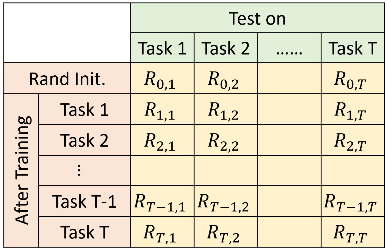
$R_{i, j}$: after training task $i$, performance on task $j$.

If $i > j$: after training task $i$, does task $j$ be forgot.

If $i < j$: task $j$ has not been learned yet, can we transfer the skill of task $i$ to task $j$.

Evaluation method:

$\text{Accuracy} = \frac{1}{T}\sum^T_{i=1}R_{T,i}$，即在机器学完所有任务后，评估其在之前任务上的表现。
$\text{Backward Transfer} = \frac{1}{T-1}\sum^{T-1}_{i=1}R_{T,i}-R_{i,i}$，即比较机器在学完所有任务后在某个任务上的表现与刚学完那个任务时的表现，从而评估当前遗忘的程度。这个值通常是负的，因为目前还是避免不了机器的遗忘，更不用提能够触类旁通使后来的表现比之前还有所提升。
$\text{Forward Transfer} = \frac{1}{T-1}\sum^{T}_{i=2}R_{i-1,i}-R_{0,i}$，即在还没有看到某个任务时，机器依照之前学习过的任务可以对该任务学出什么样的结果。

Regularization-based Approach

Why Catastrophic Forgetting?

当模型在新任务上训练时，共享的权重会被更新以最小化新任务的损失。这些更新可能会破坏之前学到的、对旧任务有用的权重配置，导致遗忘。所以可能解决的办法是对参数加一些限制。

Basic idea: Some parameters are important to the previous tasks, so only change the unimportant parameters.

The new loss function is $L'(\boldsymbol{\theta}) = L(\boldsymbol{\theta}) + \lambda\sum_ib_i(\theta_i - \theta^b_i)^2$

$L'(\boldsymbol{\theta})$ is the loss function to be optimized, $L(\boldsymbol{\theta})$ is the loss function for current task, $\theta_i$ is the parameters to be learning, $\theta^b_i$ is the parameters learned from previous tasks, $i$ means the $i$-th parameter of $\boldsymbol{\theta}$ or $\boldsymbol{\theta^b}$, $b_i$ is how important the parameter $\theta^b_i$ is. If $b_i$ is large, indicating that we hope $\theta_i$ will be as close as possible to $\theta^b_i$, i.e., $\theta^b_i$ is important.

$\boldsymbol{\theta}$ should be close to $\boldsymbol{\theta^b}$ in certain directions.

$b_i$ 的值通常是人为设定的，一个可能的做法是在模型训练好后观察 $\boldsymbol{\theta^b}$ 在各个方向上移动是否对 loss 有明显的影响，从而决定 $b_i$ 的大小。$b_i$ 的值趋于 0，意味着对参数 $\theta_i$ 的更新没有限制，会造成 Catastrophic Forgetting，导致遗忘掉旧任务；$b_i$ 的值趋于无穷大，意味着参数 $\theta_i$ 没有被更新，会造成 Intransigence，导致没有学到新任务。

设定 $b_i$ 的方法：Elastic Weight Consolidation (EWC), Synaptic Intelligence (SI), Memory Aware Synapses (MAS), etc.

Memory Reply

在训练旧任务的 classifier 时同时训练一个 generator，这个 generator 的任务是学习并生成旧任务的数据分布，然后在训练新任务时把这些生成的数据喂给新的 classifier 来避免 Catastrophic Forgetting。挑战在于需要额外的计算资源和保证生成数据的质量。

P.S. 上述只是 LLL 的其中一种情景，更多请参照 Three scenarios for continual learning。

P.S. 改变任务学习的顺序也会影响结果。研究哪种才是正确的顺序是 Curriculum Learning 关注的问题。Curriculum Learning 的基本原理是模仿人类的学习过程，即先从简单的任务（样本）开始学习，逐渐过渡到更复杂的任务（样本）。

13. Network Compression

Deploying ML models in resource-constrained environments.

Network Pruning

Networks are typically over-parameterized.

$$ \text{Pre-trained Network (Large)} \longrightarrow \text{Evaluate the Importance} \longrightarrow \text{Remove Parameters (or Neurons)} \longrightarrow \text{Fine-tune} \longrightarrow \text{Re-evaluate} \xrightarrow[]{\text{After several loops}} \text{Smaller Network} $$

Evaluate the Importance:

Importance of a weight: absolute values, LLL $b_i$, etc.
Importance of a neuron: the number of times it wasn’t zero on a given data set, etc.

After pruning, the accuracy will drop (hopefully not too much). So we need to fine-tune on training data for recover. After fine-tuning, we can re-evaluate the importance and do the loop many times. Notably, don’t prune too much at once, or the network won’t recover.

If we use weight pruning, there may be a practical issue. Because the nerwork architecture will become irregular, resulting in it being hard to implement (e.g., by PyTorch) and hard to speedup by GPU (hard to do matrix multiplication). 所以实际上做的时候为了可行性也是把 pruned weight 设为 0，而不是不存在，但是这样 network 其实并没有变小，速度也没有变快。

If we use neuron pruning, it will be easy to implement and speedup. 比如在 PyTorch 中只需要改输入和输出的 dimension 即可。

Why Pruning? - Lottery Ticket Hypothesis

首先随机初始化一个大的 Network 的参数，然后训练它并经过 Pruning 后可以成功得到一个小的 Network，再将这个小的 Network 的参数变成随机初始化的，然后训练这个小的 Network 发现训练不起来。但是，如果这里小的 Network 随机初始化的参数用的是相对应的之前大的 Network 随机初始化的那个参数，反而就能够成功训练。所以，可以解释为这一组能够成功训练的随机初始化参数就是抽到的那个能够中奖的彩票，所以如果重新随机初始化，就很难再抽到了。因此，Network 可以从大变小，但从小变大很难达到同样的表现。

Knowledge Distillation

Knowledge Distillation 中有一个大的 Network 叫做 Teacher Network 和一个小的 Network 叫做 Student Network。这里的 Student Network 是要根据 Teacher Network 来学习的。具体来说，给 Teacher Network 一个输入，它会给出一个输出，然后给 Student Network 同样的输入，要求它的输出要和 Teacher Network 的输出越接近越好（minimize cross-entropy）。这里的 Teacher Network 可以不仅仅是单一的 Network，也可以是 N 个 Network 的 Ensemble。

Temperature for softmax

\[y'_i = \frac{exp(y_i)}{\sum_jexp(y_j)} \longrightarrow y'_i = \frac{exp(y_i/T)}{\sum_jexp(y_j/T)}\]

如果 $T > 1$，可以让原本的输出分布更平滑一点。例如用原本的 softmax，如果是 $y_1 = 100, y_2 = 10, y_3 = 1$，那么经过 softmax 后的输出为 $y'_1 = 1, y'_2 \approx 0, y'_3 \approx 0$，按照这样的结果 Student 就无法从 Teacher 那里学到各个类别之间不同的程度有多大，而是跟直接从正确答案学是一样的。但是如果加上 Temperature，令 $y_1/T = 1, y_2/T = 0.1, y_3/T = 0.01$，softmax 的输出就会变成 $y'_1 = 0.56, y'_2 = 0.23, y'_3 = 0.21$，分类结果的排序不会变但是会变得平滑，这样 Student 会学得更好。$T$ 是一个 hyperparameter，也不能设太大，否则所有 class 的分数就会变得差不多。

也可以拿 softmax 前的输出做训练，或者 Network 的每一层的输出都可以拿来做训练，比如 Teacher Network 有 12 层，Student Network 有 6 层，可以让 Student 的第 6 层像 Teacher 的第 12 层，Student 的第 3 层像 Teacher 的第 6 层，等等，这样比较多的限制往往会得到更好的结果。

如果 Student 和 Teacher 差太多的话，还可以创建一个或多个中间大小的网络来进行逐步学习，这些网络介于大型的 Teacher Network 和小型的 Student Network 之间，先让中间网络学习 Teacher，再让 Student 学习这个中间网络。

Parameter Quantization

Storing each weight with fewer bits, so it can decrease the size of the model and reduce the use of computational resources.
Weight Clustering. 对模型增加了限制，可能会防止过拟合，从而提升模型的表现（Binary Weights）。
Represent frequent clusters by less bits, represent rare clusters by more bits.

Architecture Design

Depthwise Separable Convolution

Depthwise Convolution

有几个 channel 就有几个 filter，且每个 filter 只负责一个 channel（标准的 CNN 中 filter 的 channel 数需要与作为输入的 feature map 的 channel 数相同，且 filter 的数目不是固定的），但是这样就忽略了不同 channel 之间的关系。
Pointwise Convolution

用一堆 1x1 的 filter 去扫 Depthwise Convolution 后产生的 feature map（这里的 filter 同标准的 CNN 一样，它的 channel 数与要扫的 feature map 相同）来考虑不同 channel 之间的关系。

用 $I$ 代表输入的 channel 数，$O$ 代表输出的 channel 数，$k \times k$ 代表 kernel size。标准的 CNN 的参数量是 $k \times k \times I \times O$，Depthwise Separable Convolution 的参数量是 $k \times k \times I + I \times O$，所以可计算两者的比值为 $\frac{k \times k \times I + I \times O}{k \times k \times I \times O} = \frac{1}{O} + \frac{1}{k \times k}$，$O$ 通常较大（e.g., 128, 256）所以第一项很小可忽略，那么 kernel size 设为多少，Network 的大小就变为原来的几分之一。

Paper - Xception

Dynamic Computation

The network can freely adjust the computational resources it requires (e.g., different devices).

Dynamic Depth

在 Network 的每一层之间再加上一个 Extra Layer，这个 Extra Layer 的作用是根据上一个 Hidden Layer 的输出来决定目前的分类结果是什么，这样当运算资源不充足时可以让 Network 自己决定在哪一层做输出。将每一个 Extra Layer 的输出和最终输出与 ground truth 的距离（cross-entropy）加起来作为 loss $L = e_1 + e_2 + \cdots + e_N$，然后 minimize $L$ 即可。这个方法是可行的，更好的做法见 Multi-Scale Dense Network (MSDNet)。
Dynamic Width

对同一个 Network 选择不同的宽度（神经元的数量 / dims）各得到一个输出，分别计算出 cross-entropy，加起来作为 loss。更好的做法见 Slimmable Neural Networks。

14. Meta-Learning

Learning to learn 学习如何学习 and 万物皆可（在 Network 的任意 Component 中，只要是由人类设计出来的算法都可以尝试用 Meta-Learning 去学，以此作为替代品来达到相同的目标）

Chelsea Finn, Stanford, Yaqing Wang, Baidu

超参数通常在学习开始之前需要手动选择和调整（依据经验、网格搜索、随机搜索、贝叶斯优化等），需要一定的时间和计算资源，这些超参数是不是也可以是模型自己学习的呢？这就是 Meta-Learning 想要解决的问题。

手动设置超参数相当于“我”指导模型“如何去学习”，即使是像网格搜索这样的超参数调优策略，也只是相当于一个“超进化的我”在指导，整个过程依然是外部的、机械的，模型本身并没有参与超参数的选择，只是在被动的接受这些超参数。而元学习相当于让模型有能力”自己思考如何去学习“，使得模型能够根据不同的任务自动优化学习策略，即自动调整超参数，从而在新的、未知的任务上快速有效地学习和泛化（也有机会跳出思维的局限性）。

Meta-Learning Framework (Also 3 Steps)

$$ \text{Training Data (input)} \longrightarrow \text{Learning Algorithm} \ F \longrightarrow \text{Classifier} \ f^* \ \text{(output)} \\ \text{Test Data (input)} \longrightarrow \text{Classifier} \ f^* \longrightarrow \text{Class (output)} $$

Classifier $f^*$ is learned from training data, Learning Algorithm $F$ is hand-crafted. Considering $F$ is also a function, can we still learn it?

Training

What is learnable in a learning algorithm?

Gradient Descent Components (e.g., initialization parameters, optimization algorithm, network architecture). These can all be considered as “hyperparameters”, and we use $\boldsymbol{\phi}$ to represent these learnable hyperparameters.

不同的 Meta-Learning 方法其实就是基于想要学习的 hyperparameters 的不同来分类（Learning to Initialize，Learning to Optimize，Learning to Compare）。What can we “meta learn”?
Define loss function for learning algorithm $F_{\boldsymbol{\phi}}$

Loss $L(\boldsymbol{\phi})$ is a function of learnable hyperparameters $\boldsymbol{\phi}$. In traditional ML, loss function $L(\boldsymbol{\theta})$ is computed based on training data. However, loss function $L(\boldsymbol{\phi})$ is computed based on test data of training tasks in Meta-Learning. Each training task has its own training data and test data, which are typically called the support set and query set, respectively.

Feed the support set of task 1 as input into $F_{\boldsymbol{\phi}}$, which then outputs a classifier $f_{\boldsymbol{\theta^{1*}}}$. Here, $\boldsymbol{\theta^{1*}}$ represents the parameters of the classifier $f_{\boldsymbol{\theta^{1*}}}$ that are learned by $F_{\boldsymbol{\phi}}$ through minimizing the loss function $L(\boldsymbol{\theta})$ using the support set. We still don’t know whether the classifier $f_{\boldsymbol{\theta^{1*}}}$ is good or bad, so it should be evaluated on the query set of task 1. To do this, we calculate the distance or difference (e.g., cross-entropy) between the output of $f_{\boldsymbol{\theta^{1*}}}$ for each sample in the query set and the corresponding ground truth. Summing over these distances yields the loss $l^1$ of task 1. Obviously, the smaller $l^1$, the better $f_{\boldsymbol{\theta^{1*}}}$, and the better $F_{\boldsymbol{\phi}}$.

Hence, $L(\boldsymbol{\phi}) = \sum^N_{n=1}l^n$, $N$ is the number of the training tasks.
Optimization

Find $\boldsymbol{\phi}$ that can minimize $L(\boldsymbol{\phi})$, i.e., $\boldsymbol{\phi^*} = \arg \min\limits_{\boldsymbol{\phi}} L(\boldsymbol{\phi})$.

$L(\boldsymbol{\phi})$ is usually not differentiable, so we need to use RL or Evolutionary Algorithm (e.g., GA) to find $\boldsymbol{\phi^*}$. Then we’ll have a learned “learning algorithm” $F_{\boldsymbol{\phi^*}}$.

Testing

After training, we use test tasks for testing. Each test task also consists of a support set and a query set. Feed the support set of test task 1 as input into $F_{\boldsymbol{\phi^*}}$, which then outputs a classifier $f_{\boldsymbol{\theta^{1*}}}$ (i.e., it’s a within-task training). By applying this classifier to the query set of test task 1, we can obtain the predicted class. Notably, training tasks do not overlap with test tasks. Usually, the support set of test tasks only needs a little labeled data.

What can we “meta learn”?

Model Parameters (suitable for Few-shot framework)
- Initialization Parameters (Learning to Initialize)
- Embeddings / Representations (Learning to Compare)
- Optimizers (Learning to Optimize)
- Policies (Meta-RL)
Hyperparameters
- Hyperparameters Search
- Neural Architecture Search
- AutoML

Meta-Learning v.s. Few-Shot Learning

Few-Shot Learning 是目标，Meta-Learning 是达成目标的手段。

Few-Shot Learning 更专注于目标，即希望模型在只有非常少量数据（N-way K-shot, i.e., N classes and each has K examples）的情况下就可以有效的学习和预测。而 Meta-Learning 更专注于算法，即学习一种通用的 Learning Algorithm 可以帮助模型快速适应新任务。不过，目前如果想要达成 Few-Shot Learning 的目标，所使用的算法往往不是人类可以想出来的，通常都是用 Meta-Learning 得到的。

N-way K-shot 的可行性方案：

假设有 10 个端点（二分类，N=2）的数据集，先将这些端点划分为训练的端点和测试的端点（比如 8:2），然后从训练的端点中随机采样出一个端点，再从这个端点的中随机采样出 K 个样本，这样就构成了一个训练任务，每个任务都含有 N*K 个样本。不同训练任务之间的样本是可以重复的，也就是说，某些样本可能会在多个训练任务中出现。测试同理，并且在确保任务不重复的前提下，测试任务和训练任务之间的样本也是可以重复的。

Meta-Learning v.s. Machine Learning

Machine Learning	Meta-Learning
find a function $f$	find a function $F$ that is able to find $f$
Within-task Training / Testing	Across-task Training / Testing
$L(\boldsymbol{\theta}) = \sum^K_{k=1}e_k$ Sum over training examples in one task	$L(\boldsymbol{\phi}) = \sum^N_{n=1}l^n$ Sum over test (query) examples in one task and then sum over training tasks

在 Meta-Learning 上遇到同样的问题可以照搬 ML 的思路。比如解决 Overfitting 的方法就可以是 Get more training tasks 或 Task augmentation。

Across-task training includes multiple within-task training and testing cycles. Across-task training and within-task training are also called “Outer Loop” and “Inner Loop”, respectively.

Episode：Meta-Learning 的一个 Episode 就是指从某个任务的支持集学习并在查询集上测试的一个完整周期（Within-task Training + Within-task Testing），无论是 Training 还是 Testing，旨在模拟快速适应新任务的过程。

Meta-Learning v.s. Multi-Task Learning

Multi-Task Learning 可以同时处理多个任务，但是也仅限于此，如果要学新的任务，训练时通常需要再次利用旧任务的所有数据。而 Meta-Learning 可以快速适应新的任务。

因此，在做 Meta-Learning 的研究时可以把 Multi-Task Learning 的结果作为 baseline。

Sadly, there are still hyperparameters when learning a learning algorithm.

希望的是暴调一波超参数后能找到一个好的 learning algorithm，它可以用在任何新的任务上，这样在新的任务上就再也不用手动调超参数了，一劳永逸。

既然如此，那 Meta-Learning 同样应该需要 Validation Tasks 来选择它的超参数（不过一些相关的文献可能并没有，可能是两种情况，一是没调超参数，二是用了测试任务来调超参数。如果模型性能良好，后者的做法是错误的会导致结果过于乐观，前者的做法则会导致结果相对较为保守，在模型性能可以接受的情况下 ok）。

Meta-Learning? Domain Adaptation? Transfer Learning? 不必拘泥于名字，DL 一直会有新的名字出现，真正应该关注的是这些名字背后所代表的含义

Learning to Initialize (Optimization-based)

初始化的好坏就好比“有的人出生就在罗马，有的人出生就是牛马”。

在传统的 DL 中，初始化参数一般都是从一个固定的分布（正态、均匀）中随机采样得到的，这可能对新的任务来说并不是一个好的出发点。因此，需要学会找到一组通用的初始化参数，经过少量数据的少量更新后即可适应新任务，即 $\boldsymbol{\phi} = \boldsymbol{\theta^0}$。

MAML (Model-Agnostic Meta-Learning), Reptile, Meta-SGD, MAML++ (How to train your MAML)

MAML

The loss function $L(\boldsymbol{\phi}) = \sum^N_{n=1}l^n(\boldsymbol{\theta^{n*}})$ is the same as the framework mentioned above, and it uses gradient descent to minimize $L(\boldsymbol{\phi})$, i.e., $\boldsymbol{\phi} \leftarrow \boldsymbol{\phi} - \eta \nabla_{\boldsymbol{\phi}} L(\boldsymbol{\phi})$.

Considering one-step training for task $n$ (i.e., we obtain the final parameters $\boldsymbol{\theta^{n*}}$ only after one update): $\boldsymbol{\theta^{n*}} = \boldsymbol{\phi} - \varepsilon \nabla_{\boldsymbol{\phi}} l^n(\boldsymbol{\phi})$

The reasons of choosing one-step training: 1) Fast; 2) Limited training data; 3) This is the objective of MAML; 4) You can still update many times when testing.

Implementation:

Sample a training task $a$ (or a task mini-batch), and after one update ($\boldsymbol{\theta^{a*}} = \boldsymbol{\phi^0} - \varepsilon \nabla_{\boldsymbol{\phi^0}} l^a(\boldsymbol{\phi^0})$), we can obtain $\boldsymbol{\theta^{a*}}$ from $\boldsymbol{\phi^0}$;
Update once more, we can obtain the gradient $\nabla_{\boldsymbol{\theta^{a*}}} l^a(\boldsymbol{\theta^{a*}})$ when parameter is $\boldsymbol{\theta^{a*}}$, $- \nabla_{\boldsymbol{\theta^{a*}}} l^a(\boldsymbol{\theta^{a*}})$ is the direction of $\boldsymbol{\phi^0}$ update, $l^a(\boldsymbol{\theta^{a*}})$ is used to calculate $L(\boldsymbol{\phi^0})$.
Update $\boldsymbol{\phi^0}$ by gradient descent ($\boldsymbol{\phi^1} = \boldsymbol{\phi^0} - \eta \nabla_{\boldsymbol{\phi^0}} L(\boldsymbol{\phi^0})$), we can obtain $\boldsymbol{\phi^1}$.
Sample another training task $b$ to update $\boldsymbol{\phi^1}$ to $\boldsymbol{\phi^2}$.

因为用 $\nabla_{\boldsymbol{\phi}}$ 来更新参数时需要计算二次微分，所以 MAML 使用了一阶近似（first-order approximation）来简化计算（直接令二阶微分项的值为 0，得 $\nabla_{\boldsymbol{\phi}} = \nabla_{\boldsymbol{\theta^{n*}}}$），这个变种算法被称为 FOMAML (First-Order MAML)。

Why MAML is good? 论文 ANIL (Almost No Inner Loop) 提出了两种可能：1）Rapid Learning（MAML 找到的通用的初始化参数很 powerful，因此可以快速地找到每个任务所对应的好的初始化参数）；2）Feature Reuse（MAML 找到的通用的初始化参数已经很接近每个任务所对应的好的初始化参数），并认为是第二种可能。

MAML v.s. Transfer Learning (Pre-trained Model) Timestamp - 6:27

对于 MAML，我们并不关心我们要找的初始化参数 $\boldsymbol{\phi}$ 在训练任务上的表现如何，我们关心的是用 $\boldsymbol{\phi}$ 训练出来的 $\boldsymbol{\theta^*}$ 的表现如何。例如 $\boldsymbol{\phi}$ 可能在训练任务 $n$ 上表现不好，但是却可以很容易地通过 gradient descent 找到一个让 $l^n(\boldsymbol{\theta^{n*}})$ 很小的 $\boldsymbol{\theta^{n*}}$。（潜力 / 读博）

对于 Transfer Learning（$L(\boldsymbol{\phi}) = \sum^N_{n=1}l^n(\boldsymbol{\phi})$），我们要找的初始化参数 $\boldsymbol{\phi}$ 需要可以同时在所有的训练任务上都表现好，但并不能保证用 $\boldsymbol{\phi}$ 去训练后一定会在每个任务上都能得到好的 $\boldsymbol{\theta^{n*}}$（有可能在某个任务上会卡在 local minima）。（即战力 / 工作）

Reptile

采样一个训练任务 $a$，Reptile 由 $\boldsymbol{\phi^0}$ 到 $\boldsymbol{\theta^{a*}}$ 的过程可以 update 很多次（MAML 通常是一次），最终两者直接连线的方向就是 $\boldsymbol{\phi^0}$ 到 $\boldsymbol{\phi^1}$ 的更新方向。然后再继续采样并更新。

FOMAML、Reptile 和 Pre-train 三者参数更新的比较：

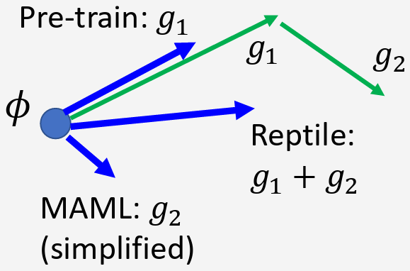
Meta-SGD

在 MAML 中，模型参数在内循环中的更新是固定的学习率 $\alpha$，而在 Meta-SGD 中，每个参数都会学习一个专属的学习率 $\alpha_{\boldsymbol{\theta}}$，即 $\boldsymbol{\theta^*_i} = \boldsymbol{\phi} - \alpha_{\boldsymbol{\phi}} \odot \nabla_{\boldsymbol{\phi}} \mathcal{L}_i(\boldsymbol{\phi})$。[^符号说明]但是这样做效率并不高，相当于学了两倍的参数。

MAML + BERT

MAML learns the initialization parameters $\boldsymbol{\phi}$ by gradient descent, but $\boldsymbol{\phi}$ itself also needs initialization. Therefore, BERT can provide $\boldsymbol{\phi^0}$ for MAML.

通常，BERT 找初始化参数（预训练）的目标是让模型学习通用的语言理解能力，这与下游任务的目标存在一定差异，导致 BERT 找到的初始化参数 $\boldsymbol{\phi}$ 不一定完全适用于下游任务（learning gap）。但是 MAML 找初始化参数的目标就是要在目标任务上具有好的表现，缺点是需要有标记的训练任务。两者各有利弊，结合或许更好（BERT + MAML > BERT 在训练数据较少时效果更显著；MAML 的 $\boldsymbol{\phi^0}$ 用 BERT 初始化也比 train from scratch 更好）。

大师的综述（2022）：Meta Learning for Natural Language Processing: A Survey 3-stage Initialization

Learning to Optimize

在传统的 DL 中，模型的训练通常依赖于标准的优化算法（e.g., SGD, Adam）来调整模型参数，以最小化损失函数。但是这些优化算法都是人思考出来的（即预先设计好的），”Learning to Optimize” 旨在让机器自己学习一种优化算法，从而可以根据具体任务的需求自动调整优化策略，即 $\boldsymbol{\phi} = \text{Optimizer}$。

LSTM (Learning to learn by gradient descent by gradient descent)

Learning to Compare (Metric-based)

Metric-based Video1, Video2, Video3, Video4

前面的做法都是将训练和测试分为两个阶段，即 Learning Algorithm $F$ 先用 Training data 训练输出 $f^*$，然后再用 $f^*$ 做测试（$F$ 负责学习，$f^*$ 负责分类）。而 Learning to Compare 的做法是将训练和测试合并为一个阶段，即将 Training data 和 Test data 都作为 $F$ 的输入，然后学习和分类都由 $F$ 负责（训练 $F$ 理解样本间的相似性或差异性，并利用这种理解来直接对新样本进行分类）。

$$ \text{Training Data + Test Data (input)} \longrightarrow \text{Learning + Classification} \ (F) \longrightarrow \text{Class (output)} $$

Siamese Network

Siamese Network Siamese Network 实际上是一个 Binary Classification 的问题。

graph LR
    A(Compound A<br>Class: Active) -->|Molecular<br>Representation| ML1(Machine Learning<br>Network)
    B(Compound B<br>Class: Active) -->|Molecular<br>Representation| ML2(Machine Learning<br>Network)
    ML1 --> E1(Embedding)
    ML2 --> E2(Embedding)
    E1 --> D("Similarity / Distance<br>(e.g., Cosine Similarity, Euclidean Distance,<br>Triplet Loss)")
    E2 --> D
    D --> O("Score<br>(Same Class, High Score;<br>Different Class, Low Score)")

如果两个输入的模态相同 / 相似，可以考虑让两个 ML Network 之间共享参数。

Siamese Network 将两个输入映射到同一个嵌入空间中，通过学习将相同的样本映射到空间中的相近点，将不同的样本映射到远离的点，从而可以用于判断两个输入是否相似。因此，Siamese Network 学出来的 Embedding 会包含用于分类的关键信息，而忽略那些不重要的信息（比如用于人像识别时的背景信息）。

Triplet Loss：经常用在如何从输入数据中提取有用的特征以进行比较的场景中。一个 Triplet 由三部分组成：Anchor（参考数据点），Positive（与 Anchor 属于同一类别的数据点）和 Negative（与 Anchor 属于不同类别的数据点）。其思想是让 Positive 的嵌入更接近 Anchor 的嵌入，而 Negative 的嵌入更远离 Anchor 的嵌入，在训练过程中模型学习生成能够区分不同类别数据的嵌入。其公式如下：
\[L(A, P, N) = \max(\Vert f(A) - f(P) \Vert^2_2 - \Vert f(A) - f(N) \Vert^2_2 + margin, 0)\]
$f$ 表示嵌入函数，将输入数据映射到嵌入空间，$\Vert \cdot \Vert_2$ 表示 L2 范数（Euclidean Distance），$A$ 表示 Anchor，$P$ 表示 Positive，$N$ 表示 Negative，$margin$ 是一个超参数，用于确保 $A$ 和 $N$ 之间的距离至少比 $A$ 和 $P$ 之间的距离大一个特定的值，即确保同一类别的数据点总是更接近，用公式表示就是要满足 $\Vert f(A) - f(P) \Vert^2_2 + margin < \Vert f(A) - f(N) \Vert^2_2$，此时，Loss 为 0。应用 Triplet Loss 时，往往需要构造难以区分的 Triplet（不容易满足上述不等式）使训练更具有挑战性，从而能够有效推动模型的学习。

Prototypical Network

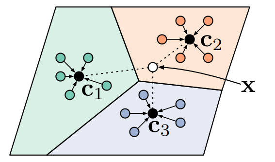
对于每个 class，计算输入点的 embedding 的平均值（叫做 prototype），计算测试点与各个 prototype 的距离，将其分类到距离最近的 prototype 所在的 class。

GPT-4 Summary

Prototypical Networks 特别设计用于处理 few-shot learning 问题，其核心思想就是利用少量的样本（即“few shots”）来学习每个类别的代表性特征，称为原型（prototype）。一、原理和应用 Prototypical Networks 通过以下步骤实现 few-shot learning： 1. 支持集（Support Set）：在每次训练或测试过程中，模型首先接收一个支持集，其中包含每个类的少量样本。这些样本数目通常很小，比如在 5-shot learning 的设置中，每个类有 5 个样本。 2. 计算原型：对于每个类，模型计算支持集中所有样本的嵌入（embedding）的平均值，这个平均值形成了该类的原型。这种方法假定类内的样本是相似的，因此通过平均化可以得到一个好的类表示。 3. 比较距离：在测试阶段，对于每一个测试样本（来自查询集，即 Query Set），模型计算其与每个类的原型之间的距离。距离可以使用欧氏距离或其他相似的度量。 4. 分类决策：测试样本被分类到与其最近的原型所代表的类别。二、动机和优势这种方法在 few-shot learning 场景中非常适用，因为它不需要大量的样本来进行有效的学习。通过集中于计算每个类的原型，Prototypical Networks 能够有效地总结和利用有限的数据信息。此外，原型的计算和距离的比较都是计算上非常高效的操作，使得模型即便在样本极少的情况下也能快速运作。三、挑战尽管 Prototypical Networks 在多个 few-shot learning 任务中表现出色，它仍然面临一些挑战，例如： 5. 类内差异性：如果一个类内部的样本差异较大，单一的原型可能不足以捕捉全部的类特性。 6. 特征表示的质量：模型的性能很大程度上依赖于输入样本特征的质量和表达能力。因此，如何有效地学习和提取特征显得尤为重要。四、总结 Prototypical Networks 通过在支持集上为每个类计算原型，并在查询集上进行分类，为 few-shot learning 提供了一种简洁而有效的解决方案。这种方法通过聚焦于类原型的学习，使得即使在样本极其有限的情况下也能进行有效的学习和预测。

Weighted Prototypical Network may be better?

Matching Network

相比于 Prototypical Network，Matching Network 考虑输入数据之间也许是有顺序关系的，因此它的嵌入函数是 Bidirectional LSTM。但 Prototypical Network 认为改变输入数据的顺序不应该影响最后的输出结果。Prototypical Network 是后提出的，且其表现和速度都更好。

Relation Network

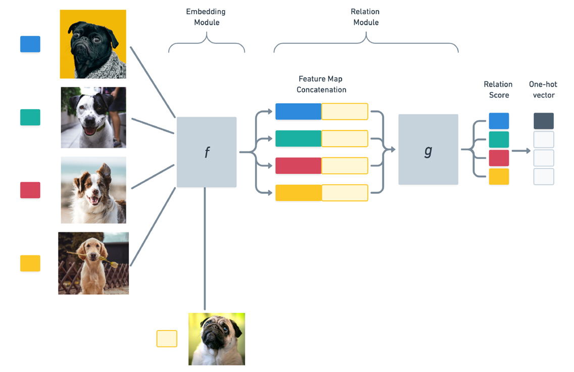
前面提到的 Network 计算训练样本和测试样本之间 Similarity 的方法都是由人定的，Relation Network 提出如何计算 Similarity 应该由一个 Network $g$ 自己学出来，$g$ 接受训练样本和测试样本拼接的 embedding 作为输入。这里的 $g$ 和嵌入函数 $f$ 是一起被学出来的。

Imaginary Data

Low-Shot Learning from Imaginary Data

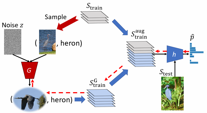
在训练数据后加一个 generator，对训练数据进行域内变换，相当于做 data augmentation，将增强后的训练数据和原训练数据合并再与测试数据输入到 Network $F$ 中，这里的 generator 是和 $F$ 一起学出来的。

像 Siamese Network 等 Learning to Compare 的 $F$ 的架构其实都算是经过特定设计的，那 $F$ 可不可以是一个 Generalized Network 呢？

MANN, SNAIL

Neural Architecture Search

在 Meta-Learning 中，如果 $\boldsymbol{\phi} = \text{Network Structure}$，那就相当于在做 Neural Architecture Search (NAS)。对于 $\boldsymbol{\phi^*} = \arg \min\limits_{\boldsymbol{\phi}} L(\boldsymbol{\phi})$，因为网络架构 $\boldsymbol{\phi}$ 是不可微分的，所以要用 RL 硬做。把 $\boldsymbol{\phi}$ 当作是 RL 的 Agent，Agent 的输出是网络架构相关的超参数（e.g., 层数，每层的神经元数，kernel size），目标是训练 Agent 能够最大化 Reward，这里的 Reward 就设为 $-L(\boldsymbol{\phi})$，所以就可以相当于是最小化 $L(\boldsymbol{\phi})$。具体操作上，根据 Agent 的输出的超参数能构建一个网络，用训练任务的支持集去训练这个网络，然后以其在查询集上的 Accuracy 作为 Reward 来训练 Agent。

Data Processing

Meta-Learning 也可以用于 Data Processing，即 $\boldsymbol{\phi} = \text{Data Processing Strategy}$。

Data Augmentation：让机器学习如何在不同的任务上做最有效的 Data Augmentation（类型、程度、不同类型的顺序等）。

AutoAugment: Learning Augmentation Policies from Data
Sample Reweighting：让机器学习根据数据的特性自己决定给予不同的样本以不同的权重，也许可以用在不平衡的数据集上。

Learning to Reweight Examples for Robust Deep Learning

Meta-Weight-Net: Learning an Explicit Mapping For Sample Weighting

Beyond Gradient Descent

上述所提到的 Meta-learning 的方法都是基于 Gradient Descent 来学习其中的一个 Component，有没有可能让机器舍弃掉 Gradient Descent，发明出全新的 Learning Algorithm，即 $F_{\boldsymbol{\phi}}$ 仅需输入即可给出输出 $f_{\boldsymbol{\theta^*}}$。

Meta-Learning with Latent Embedding Optimization

AutoML

auto-sklearn

AutoML

Meta-Learning for Active Learning

优化主动学习的样本选择策略？

Meta-Reinforcement Learning

优化强化学习的策略学习过程？

RL 最耗费时间的部分在于与环境互动的过程，相当于在收集数据，所以可以用 Meta-Learning 的方法做 Few-Shot。

A Survey of Meta-Reinforcement Learning

Papers With Code - Meta Reinforcement Learning

Lil’Log - Meta Reinforcement Learning

Meta-Learning for GNN

Meta-Learning with Graph Neural Networks: Methods and Applications

Graph Meta Learning via Local Subgraphs

Graph Sampling-based Meta-Learning for Molecular Property Prediction

Few-Shot Learning on Graphs: from Meta-learning to Pre-training and Prompting

Meta Learning With Graph Attention Networks for Low-Data Drug Discovery

Meta-Transfer Learning

Meta-Transfer Learning for Few-Shot Learning

15. Transfer Learning

Source Data and Target Data are Both Labeled

Fine-tuning

There are a large amount of source data (not directly related to the task) and only a little target data. Training a model by source data as the initialization, then fine-tuning the model by target data. But be careful about overfitting.

Conservative Training

限制用 target data 微调后的模型与用 source data 预训练的模型它们的输出或参数不要差得太多。
Layer Transfer

从预训练的模型中 copy 一些 layers，然后用 target data 去训练剩余的 layers（防止过拟合）。问题是哪些 layer 需要被 transferred（copied）？根据任务特性来定，可以 copy 的 layer 一般是能够识别通用的特征。

Multi-Task Learning

Fine-tuning 只关心在 target domain 上做的好不好，而 Multi-Task Learning 则同时关心 source domain 和 target domain。如果各个 task 的 input feature 是相同的，那么可以在 NN 的前几层同时使用这些 task 的数据来做训练，需要保证这些 task 之间具有共通性。如果各个 task 的 input feature 是不同的，可以先分别通过一个 NN 转移到同一个 domain 上，在这个 domain 上有些参数是可以共享的，然后再分别到一个 NN 上做分类/回归。

Source Data is Labeled but Target Data is Unlabeled

Domain-Adversarial Training

把 source data 当作 training data，target data 当作 test data，它们的 task 是一样的，但是 domain 会存在 mismatch。Domain-Adversarial Training 要做的是学一个 feature extractor，来消除 source domain 和 target domain 之间的 mismatch（通过 t-SNE 降维可以观察到不同 domain 混合在一起）。具体做法是把 feature extractor 的输出输入到一个 domain classifier 里来判断输入的 feature 来自于哪个 domain（即 feature extractor 输出的 feature 要能够使得 domain classifier 无法准确判断其来自于哪个 domain）。feature extractor 输出的 feature 同时还要保证 label predictor 的结果要好。训练时，feature extractor 要试图最小化 label predictor 的损失函数，同时最大化 domain classifier 的损失函数。

Zero-Shot Learning

把 source data 当作 training data，target data 当作 test data，但是它们的 task 是不一样的。在 Zero-Shot Learning 中，需要 Represent each class by its attributes，所以会有一个 database 来储存 class 和 attribute 之间的映射关系（attribute 需要足够多），因此，NN 输出的不再是 class 而是 attribute（一个由 0 和 1 组成的向量代表各个 attribute 有无），测试时就可以 find the class with the most similar attributes。

Attribute Embedding

通过一个 NN $f$ 将 input $x^n$ 映射到一个 embedding space，同样地，attribute $y^n$ 也通过一个 NN $g$ 被映射到同一个 embedding space，希望 $f(x^n)$ 和 $g(y^n)$ 越接近越好。其 loss function 的形式为 $f^*, g^* = \arg \min\limits_{f,g} \sum\limits_n \max(0, k - f(x^n) \cdot g(y^n) + \max\limits_{m \ne n}f(x^n) \cdot g(y^m))$，如果想要 loss 为 0，则有 $f(x^n) \cdot g(y^n) - \max\limits_{m \ne n}f(x^n) \cdot g(y^m) > k$，若此式成立，需要配对的 $f(x^n)$ 和 $g(x^n)$ 接近且其他不配对的 $f(x^n)$ 和 $g(y^m)$ 远离。

16. GNN

A node can learn the graph structure from its neighbors directly and indirectly. It can be considered as a kind of convolution, i.e., each convolution is equivalent to performing a message passing and an update for the node feature.

The problem is how to embed the node into a feature space using convolution.

Spatial-based Convolution

直接在图的空间结构上操作，通过聚合（Aggregate）邻居节点的特征信息来更新当前节点的特征，比较灵活，适用于动态图或需要灵活定义邻居聚合方式的场景。

Aggregation 更新的是每个节点的特征，但是如果想要的是整个图的特征（比如化学分子），就需要做 Readout 把所有节点的特征集合起来以代表整个图。

Aggregation	Method
Sum	NN4G
Mean	DCNN, DGC, GraphSAGE
Weighted Sum	MoNET, GAT, GIN
Max Pooling	GraphSAGE
LSTM	GraphSAGE

Implementation

分子在输入层时，首先通过用各种不同的化学性质来表示 node feature（RDKit / DGL-LifeSci），然后通过嵌入层让 node feature 变成 embedding（用 weight 做 transformation，嵌入层的权重矩阵大小为 [num_nodes, embedding_dim]），然后再通过任意次的 aggregation 来更新 embedding，最后做 Readout。（对于分子性质预测，一般用的是最后 readout 得到的图嵌入作为 ML 模型的输入去做下游的 Graph Classification / Regression，maybe 也可以端到端直接由 GNN 给出预测）

像 GCN、GAT 这种作为网络的一层，可以考虑交替使用，从而允许模型在不同的层级上利用基于结构的特征聚合和基于注意力的特征聚合；或者合并它们的输出，提供更丰富的节点表示。

GIN 适合捕捉全局图结构，可能适用于整体分子的性质；GCN、GAT 可能适用于理解分子中特定的局部结构。

常用：GCN, GAT, GIN, GraphSAGE, AttentiveFP

GraphSAGE

Paper

GraphSAGE (SAmple and aggreGatE) learns how to embed node features from neighbors. GraphSAGE 是归纳式（Inductive）的，它不是学习固定的图中每个节点的嵌入，而是学习一个嵌入函数，从而能够为未见过的节点生成嵌入，提高了泛化能力。

Sample: Ignore the order of neighbors for nodes
Aggregation: Mean, Max Pooling, or LSTM

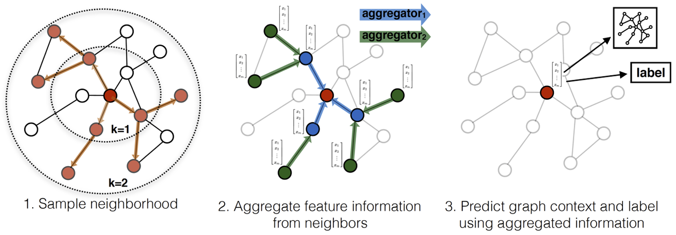
GAT

Paper

(Graph Attention Network) 不仅要做 Weighted Sum，并且 Weighted Sum 的 weight 是通过 Self-attention 让模型自己学到的。

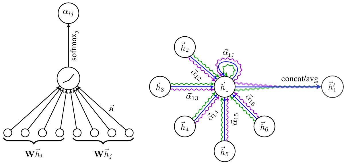
Note: 1) The weight vector $\vec{\mathbf{a}}$ represents the parameters of a single-layer feedforward neural network; 2) The aggregated features from each head (different arrow styles denote independent heads, 3 heads here) are concatenated or averaged to obtain $\vec{h'_1}$; 3) The multi-head attention allows for the parallel use of multiple independent attention within the same layer to update node features. 4) Terminology: The notation $\Vert$ denotes the concatenation of vectors, $\mathbf{W}$ denotes the weight matrix, $\mathbf{W} \vec{h_i}$ denotes the linear transformation of $\vec{h_i}$.

GIN

Injection（单射）：从集合 $A$ 到集合 $B$ 的映射中，$A$ 中的每个元素都映射到 $B$ 中的唯一元素，不会有两个不同的元素映射到同一个元素，保证了一一对应的关系。即假设有一个函数 $f: X \rightarrow Y$，如果对于任意的 $x_1, x_2 \in X$，只要 $x_1 \neq x_2$，就有 $f(x_1) \neq f(x_2)$，那么函数 $f$ 就是单射的。

Surjection（满射）：从集合 $A$ 到集合 $B$ 的映射中，对于集合 $B$ 中的每个元素，都至少存在一个集合 $A$ 中的元素与之对应。即假设有一个函数 $f: X \rightarrow Y$，如果对于任意的 $y \in Y$，都存在一个 $x \in X$ 使得 $f(x) = y$，那么函数 $f$ 就是满射的。

Bijection（双射）：集合 $A$ 中的每个元素都与集合 $B$ 中的唯一元素相对应，并且集合中 $B$ 的每个元素也都与集合 $A$ 中的唯一元素相对应，即同时满足了单射和满射的条件。

Multiset: a set with possibly repeating elements.

Graph Isomorphism（图同构）：研究两个图在结构上是否完全相同，即两个图是否可以通过重新标记节点后变得无法区分。具体来说，给定两个图 $G_1 = (V_1, E_1)$ 和 $G_2 = (V_2, E_2)$，如果存在一个双射 $f: V_1 \rightarrow V_2$，使得对于 $G_1$ 中任意两个节点 $u$ 和 $v$，它们之间存在边的条件是当且仅当 $f(u)$ 和 $f(v)$ 在 $G_2$ 中存在边，则这两个图是同构的。图同构保留了节点和边的连接方式，但不一定保留节点或边的标签。（下图为一个简单的图同构例子，映射关系为：$\text{A} - 3; \text{B} - 1; \text{C} - 2; \text{D} - 5; \text{E} -4$）

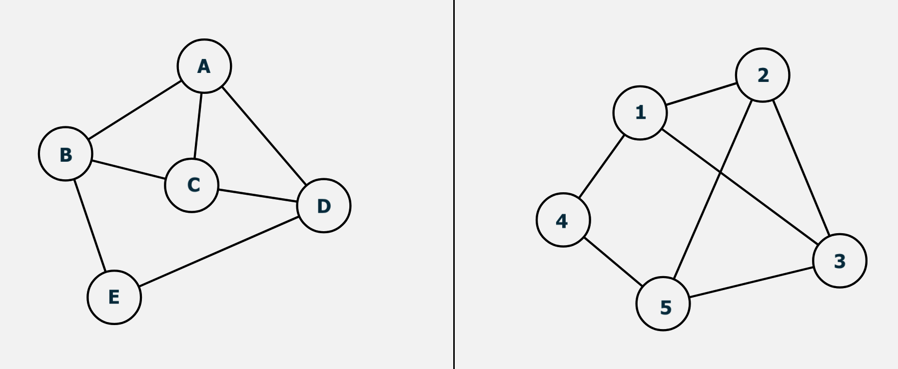
Weisfeiler-Lehman test：是一种用于检测两个图是否同构的算法。WL test 基于 rooted subtree（也可以看作是一种 subgraph）考虑了每个节点及其邻域，通过迭代的方式，逐步更新图中每个节点的标签，直到达到一定的迭代次数或者所有节点的标签不再发生变化时，通过比较两个图中节点的标签分布是否相同来判断这两个图是否同构。WL test 一般是 1-dimensional 形式的，即在迭代过程中只考虑了每个节点自身及其一阶邻居的信息来更新节点的标签，并没有考虑更高阶的邻域（neighborhood）信息。下图为一个以 node 1 为根节点 height 为 2（迭代两次）的 rooted subtree。Weisfeiler-Lehman Graph Kernels

在 GNN 的研究中，WL 测试常被用来衡量 GNN 模型的性能，一个 GNN 模型如果能够模拟 WL 测试的行为，那么就可以认为该模型能够很好地捕捉图的结构信息（特征提取 / 生成图的表示），从而应用于更广泛的下游任务。WL test - GNN的性能上界

Paper

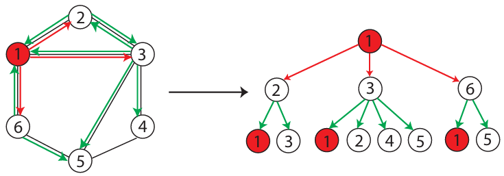
GIN (Graph Isomorphism Network) 的理论框架：

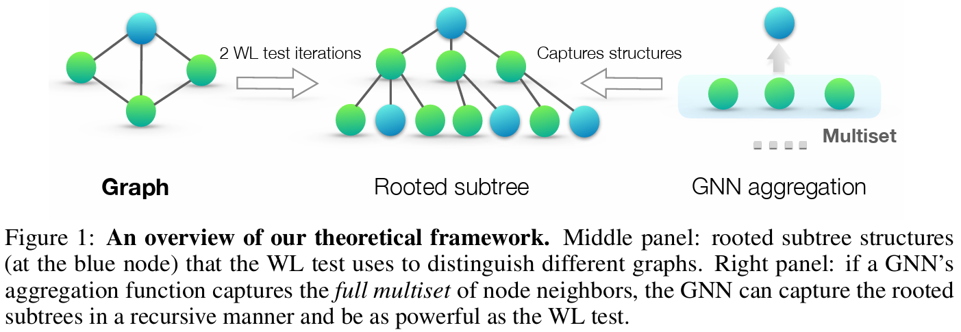
一个好的 GNN 算法的聚合节点的邻域信息生成节点新的 representation 的过程应该是单射的，即永远不会将两个不同的邻域映射得到相同的 representation。对于 GIN 来说，旨在通过训练可以学习到一个近似单射的函数，使得不同的节点及其邻域信息能够被映射到特征空间中的唯一向量，即 $h^k_v = \phi (h^{k-1}_v, f(\{h^{k-1}_u : u \in \mathcal{N}(v)\}))$。上述公式中，$h^k_v$ 表示节点 $v$ 在第 $k$ 次迭代中的特征向量；$\phi$ 表示更新函数；$f$ 表示聚合函数，作用于 multiset（即节点 $v$ 所有邻居节点的特征向量所组成的集合）；$\mathcal{N}(v)$ 表示节点 $v$ 的邻域。

GIN 使用 MLP 来建模和学习 $f$ 和 $\phi$，使整个节点更新过程尽可能接近单射函数，而之所以用 MLP 是因为它能够近似任何连续函数的组合。$\epsilon$ 可以是一个可学习的参数或固定的标量，用于调整节点自身特征与其邻居特征之和的贡献比例。

\[h^k_v = \text{MLP}^k((1 + \epsilon^k) \cdot h^{k-1}_v + \sum_{u \in \mathcal{N}(v)} h^{k-1}_u)\]

GIN 的 readout 的做法是对于每次迭代都使用 $\text{READOUT}$ 函数来处理所有节点的嵌入，以生成该次迭代的图的嵌入，然后经过 $K$ 次迭代后，将每次迭代生成的图的嵌入拼接起来作为最终的图的嵌入 $h_G$。这样做能够在最后的输出中捕捉到图在不同阶段的信息，而不会局限于最后一个阶段。论文中也写道 “A sufficient number of iterations is key to achieving good discriminative power. Yet, features from earlier iterations may sometimes generalize better.”，所以早期迭代的图的嵌入可能也很重要，我们不应该忽视。

\[h_G = \text{CONCAT}(\text{READOUT}(\{ h^k_v \mid v \in G \}) \mid k = 0,1,\dots, K)\]

对于 aggregation 的方式，sum 可以捕捉到 multiset 中的所有元素的完整信息；mean 可以捕捉到不同元素类型的比例或分布，但忽略了元素的具体数量（重复元素），这在需要邻域的整体性质时很有用；max 只能捕捉到最大元素的信息。因此，sum 的区分能力最强。

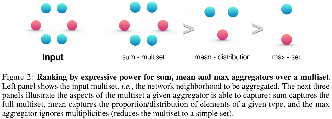
Spectral-based Convolution

傅里叶变换（Fourier Transform）的卷积定理：两个函数 $x(t)$ 和 $y(t)$ 在时域（Time Domain）的卷积等价于它们的傅里叶变换 $X(f)$ 和 $Y(f)$ 在频域（Frequency Domain）的乘积。乘积运算要比卷积运算简单得多，这可以帮助我们设计滤波器（filter），滤波器在频域中可以很简单地表示为乘一个函数。通过傅里叶变换，任何信号都可以表示为不同频率的正弦波和余弦波的线性组合。

Eigenvalue Decomposition (EVD)：对于一个矩阵 $A$，特征值分解希望找到一组特征向量 $u$ 和相应的特征值 $\lambda$，满足 $Au = \lambda u$。分解后，$A$ 可以表示为 $A = U \Lambda U^T$，$U = [u_0, u_1, \dots, u_{N-1}] \in \mathbb{R}^{N \times N}$ 是一个由特征向量组成的矩阵，$\Lambda = \text{diag}(\lambda_0, \lambda_1, \dots, \lambda_{N-1}) \in \mathbb{R}^{N \times N}$ 是一个对角矩阵，其对角线上的元素是相应的特征值。

Spectral Graph Theory

目标：需要定义一个图的傅里叶变换，才能在图上做 filter。这个傅里叶变换涉及到将信号从图的 Vertex Domain（Time Domain）转换到 Spectral Domain（Frequency Domain）。

Terminology:

Graph $G = (V,E)$, $N = \vert V \vert$ is the number of vertices.
Adjacency Matrix $A \in \mathbb{R}^{N \times N}$, $A_{i,j} = \begin{cases} 0 & \text{if } e_{i,j} \notin E \\ w(i,j) & \text{else} \end{cases}$ is the weight of the edge between vertices $i$ and $j$, and $A$ is a symmetric matrix for an undirected graph.
Degree Matrix $D \in \mathbb{R}^{N \times N}$, $D_{i,j} = \begin{cases} d(i) & \text{if } i = j \\ 0 & \text{else} \end{cases}$ is the degree of vertex $i$, $d(i)$ is equivalent to the sum of row $i$ in $A$ (i.e., $D_{ii} = \sum_jA_{ij}$), and $D$ is a diagonal matrix.
Signal on Graph $f : V \rightarrow \mathbb{R}^N$, $f(i)$ is the signal on vertex $i$. Specifically, the function $f$ maps each vertex $v \in V$ to an N-dimensional real number vector, where each dimension can represent different features or attributes of the vertex.
Graph Laplacian Matrix $L = D - A$, when performing spectral decomposition (eigenvalue decomposition) on $L$, i.e., $L = U \Lambda U^T$, the obtained eigenvalue $\lambda_i$ can be considered as the frequency of vertex $i$, while the eigenvector $u_i$ corresponding to $\lambda_i$ is the frequency-domain basis. Through these eigenvectors, it is possible to transform signals from the frequency domain back to the time domain, achieving signal reconstruction.
Nomalized Graph Laplacian Matrix $L = I - D^{-1/2}AD^{-1/2}$, it can help to preserve the structural information of the graph while reducing the influence of varying graph sizes and node degree distributions.

当将 Graph Laplacian Matrix 应用于图上的信号时，即 $Lf(v_i) = \sum_{j \in \mathcal{N}(i)} w_{i,j}(f(v_i) - f(v_j))$，这里的 $Lf(v_i)$ 是节点 $v_i$ 的拉普拉斯信号，反映的是能量的局部差异，即每个节点与其邻居之间的信号差异，但 $Lf$ 的结果还是一个向量，每一行对应一个节点。

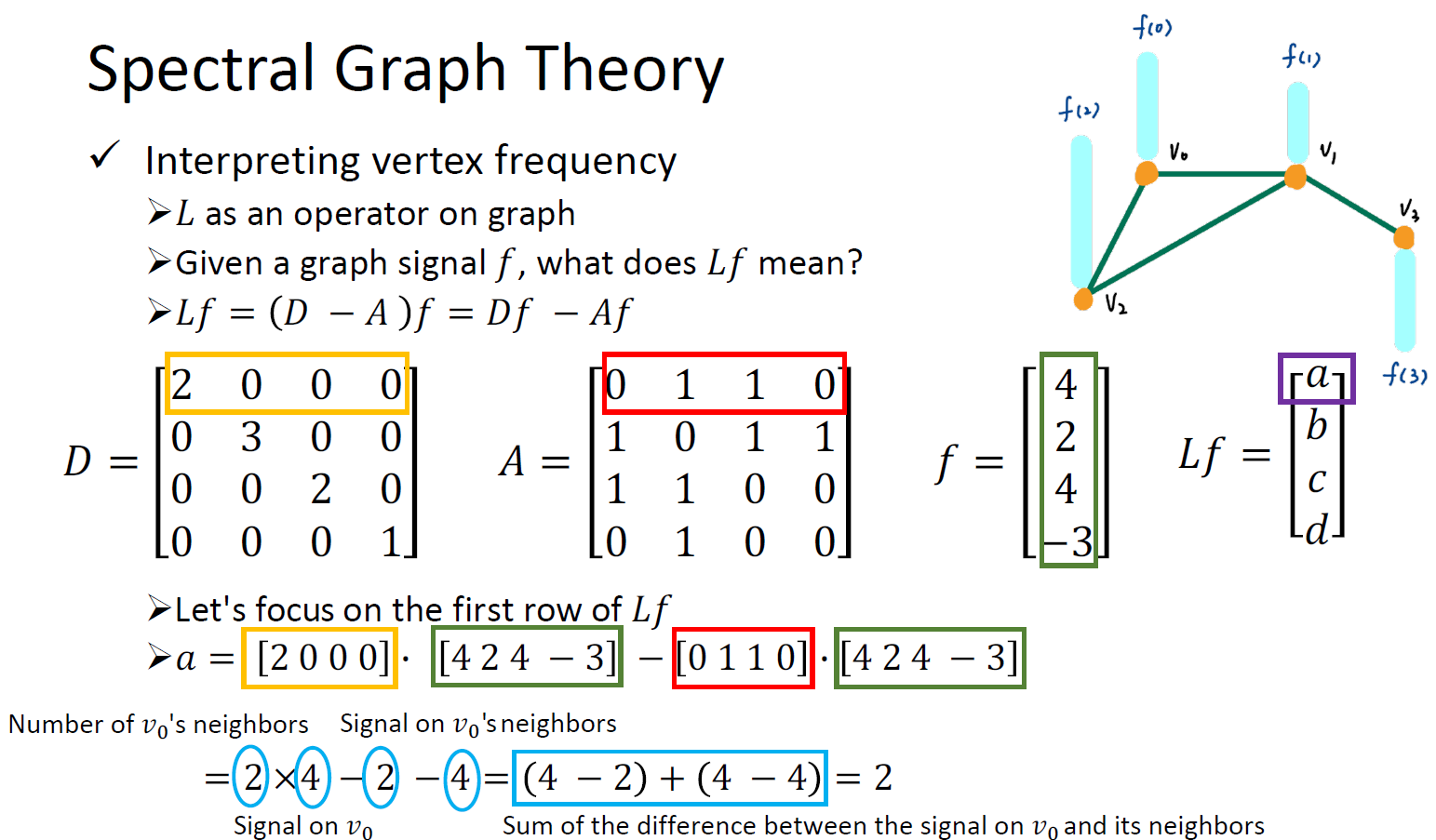
如果要计算能量的全局差异，则需要计算 $f^TLf = \frac{1}{2} \sum_{v_i \in V} \sum_{v_j \in V} w_{i,j} (f(v_i) - f(v_j))^2$，这是一个点积操作，即原信号 $f$ 的每个元素（节点自身的信号值）乘以其对应的局部差异（$Lf$）并求和。$f^TLf$ 反映了整个图的信号平滑度，如果其值小，说明信号在图上相邻节点之间变化不大，信号比较平滑。信号越平滑，则频率越低。当用 $L$ 的特征向量 $u_i$ 替换 $f$，计算 $u_i^TLu_i = \lambda_iu_i^Tu_i = \lambda_i$ 得到的是特征值 $\lambda_i$，即 $\lambda_i$ 代表了能量差异，因此 $\lambda_i$ 可以被看作是 $u_i$ 的频率大小，较小的 $\lambda_i$ 对应低频率，较大的 $\lambda_i$ 对应高频率。

图的傅里叶变换依赖于图拉普拉斯矩阵的特征值和特征向量，主要由三个步骤组成：

Transform

Graph Fourier Transform of signal $x$: $\hat{x} = U^Tx$，将原始信号从顶点域转换到谱域，可以得到信号 $x$ 在各个频率 $\lambda_i$ 上的成分（Component）大小 $u_ix$ 是多少（$U^T$ 的每一行对应一个特征向量 $u_i$，相当于信号在各个频率上的投影）。
Filter

图滤波器的频率响应（Frequency Response）描述了滤波器对于各个频率成分的增益或衰减程度，可以表示为对应于特征值 $\Lambda$ 的函数 $H(\Lambda)$，与谱域信号 $\hat{x}$ 直接相乘相当于做了卷积运算 $\hat{y} = H(\Lambda)\hat{x}$ 。
Inverse Transform

Inverse Graph Fourier Transform of signal $\hat{x}$: $x = U\hat{x}$，将谱域信号转换回顶点域，重建原始信号。如果应用了滤波器，则公式为 $y = U\hat{y}$。

因此，可以推导出 $y = U\hat{y} = UH(\Lambda)\hat{x} = UH(\Lambda)U^Tx = H(U\Lambda U^T)x = H(L)x$，所以模型需要学一个有关 $L$ 的函数 $H(L)$（即 filter），输入 $x$ 后可以得到一个经过 filter 的 $y$。如果 $H(L)$ 被参数化可以写作 $g_{\boldsymbol{\theta}}(L)$，即 $y = g_{\boldsymbol{\theta}}(L)x$。

如果 $H(L)$ 可以展开一直到 $L^N$（图有 $N$ 个顶点），会导致模型的复杂度是跟输入的图的大小有关的，我们希望的则是不管输入的图有多大都可以用同样大小的模型去训练。另外，$L^N$ 还会导致所有节点都能互相影响，而我们希望的是模型能够通过 filter 来捕获顶点的局部信息（类比 CNN 的 filter）。

ChebyNet

Paper

由 $y = g_{\boldsymbol{\theta}}(L)x = g_{\boldsymbol{\theta}}(U\Lambda U^T)x = Ug_{\boldsymbol{\theta}}(\Lambda)U^Tx$ 和 $g_{\boldsymbol{\theta}}(\Lambda) = \text{diag}(\boldsymbol{\theta})$，令 $g_{\boldsymbol{\theta}}(\Lambda)$ 是 $\Lambda$ 的多项式函数 $g_{\boldsymbol{\theta}}(\Lambda) = \sum^{K-1}_{k=0}\theta_k\Lambda^k$ ，因此可以让 $g_{\boldsymbol{\theta}}(\Lambda)$ 为 $K$-localized 且降低了复杂度。

Chebyshev Polynomial: $T_0(x) = 1, T_1(x) = x, T_k(x) = 2xT_{k-1}(x) - T_{k-2}(x), x \in [-1, 1]$

依照 Chebyshev Polynomial，有 $T_0(\tilde{\Lambda}) = I, T_1(\tilde{\Lambda}) = \tilde{\Lambda}, T_k(\tilde{\Lambda}) = 2\tilde{\Lambda}T_{k-1}(\tilde{\Lambda}) - T_{k-2}(\tilde{\Lambda})$，where $\tilde{\Lambda} = \frac{2\Lambda}{\lambda_{max}} - I, \tilde{\lambda} \in [-1, 1]$，$I$ 是指 Identity Matrix。因此，原来的多项式函数会变为 $g_{\boldsymbol{\theta'}}(\Lambda) = \sum^{K-1}_{k=0}\theta'_kT_k(\tilde{\Lambda})$，这样做会比较好算，所以整个 filter 的操作可以被写成 $y = g_{\boldsymbol{\theta'}}(L)x = \sum^{K-1}_{k=0}\theta'_kT_k(\tilde{L})x$，而模型要学的参数就是 $\boldsymbol{\theta'}$。

GCN

Paper

令 ChebyNet 的 filter 公式中的 $K = 1$，有

\[\begin{align*} y = g_{\boldsymbol{\theta'}}(L)x &= \theta'_0x + \theta'_1 \tilde{L}x \\ &= \theta'_0x + \theta'_1(\frac{2L}{\lambda_{max}}-I)x \ , \ (\lambda_{max} \approx 2) \\ &= \theta'_0x + \theta'_1(L-I)x \ , \ (L = I - D^{-1/2}AD^{-1/2}) \\ &= \theta'_0x + \theta'_1(D^{-1/2}AD^{-1/2})x \ , \ (\theta = \theta'_0 = -\theta'_1, \text{for reducing the parameters}) \\ &= \theta(I + D^{-1/2}AD^{-1/2})x \end{align*}\]

然后为每个节点加上一个自环（self-loop），即 $\tilde{A} = A + I$（对角线元素一定为 1）和 $\tilde{D}_{ii} = \sum_j\tilde{A}_{ij}$，从而有 $I + D^{-1/2}AD^{-1/2} \rightarrow \tilde{D}^{-1/2}\tilde{A}\tilde{D}^{-1/2}$，作者称之为 $renormalization \ trick$。所以 GCN 中一层的传播可以写为 $H^{(l+1)} = \sigma(\tilde{D}^{-1/2}\tilde{A}\tilde{D}^{-1/2}H^{(l)}W^{(l)})$，$\sigma$ 是激活函数，$H^{(l)}$ 是第 $l$ 层的节点特征矩阵（$x$），$W^{(l)}$ 是第 $l$ 层的权重矩阵（$\theta$），即在每一层只考虑一个顶点的直接相连的邻居（1-localize）及其自身的特征来更新该顶点的特征。

在第一层，每个节点只能捕捉到其一阶邻居和其自身的特征，在第二层，每个节点就能捕捉到其二阶邻居的特征（节点的一阶邻居的特征也更新了）。但是随着 GCN 层数的增加，每个节点的特征会越来越“全局化”，可能会导致所有节点的特征逐渐变得相似，从而失去了区分度（over-smoothing）。

Gated-GCN

Residual Gated Graph ConvNets

Benchmarking Graph Neural Networks

Graph Generation

VAE-based model: Generate a whole graph in one step

GraphVAE
GAN-based model: Generate a whole graph in one step

MolGAN
Autoregressive-based model: Generate a node or an edge in one step

Learning Deep Generative Models of Graphs
More

A Comprehensive Survey on Graph Neural Networks

New

GraphGPS

Graph Neural Networks with Learnable Structural and Positional Representations

Appendix

Hyperparameters

learning rate
no. of sigmoid
batch size
no. of hidden layers
momentum $\lambda$
RMSProp $\alpha$
CNN: kernel size, number of filters, stride, padding, pool size, pool stride, pooling type
Multi-head self-attention: numbers of head
temperature for softmax $T$

PyTorch

Features: 1) Tensor computation with GPU acceleration; 2) autograd (Automatic Differentiation); 3) PyTorch for research, TensorFlow for Production

Data Type

Data Type	dtype	tensor
32-bit floating point	torch.float	torch.FloatTensor
64-bit integer (signed)	torch.long	torch.LongTensor

Shape of Tensors

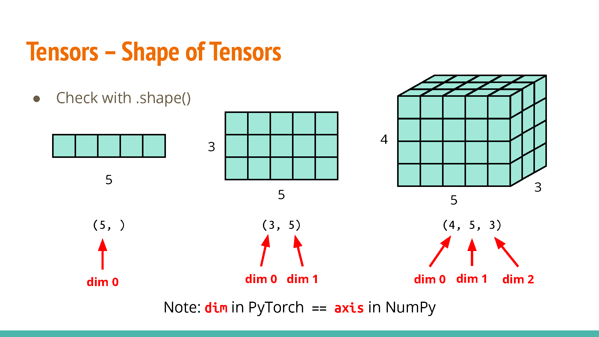
Creating Tensors

Directly from data (list or numpy.ndarray)

x = torch.tensor([[1, -1], [-1, 1]])
x = torch.from_numpy(np.array([[1, -1], [-1, 1]]))

Tensor of constant zeros & ones

x = torch.zeros([2, 2])
x = torch.ones([1, 2, 5])

Common Operations

Addition, Subtraction, Power, Summation, Mean

z = x + y
z = x - y
y = x.pow(2)
y = x.sum()
y = x.mean()

Transpose, Squeeze, Unsqueeze

>>> x = torch.zeros([1, 2, 3])
>>> x.shape
torch.Size([1, 2, 3])

# transpose
>>> x = x.transpose(0, 1)
>>> x.shape
torch.Size([2, 1, 3])

# squeeze the dimension that its size is 1
>>> x = x.squeeze(1)
>>> x.shape
torch.Size([2, 3])

# unsqueeze
>>> x = x.unsqueeze(1)
>>> x.shape
torch.Size([2, 1, 3])

Cat

# concatenate multiple tensors
>>> x = torch.zeros([2, 1, 3])
>>> y = torch.zeros([2, 3, 3])
>>> z = torch.zeros([2, 2, 3])
>>> w = torch.cat([x, y, z], dim=1)
>>> w.shape
torch.Size([2, 6, 3])

Device

Tensors & modules will be computed with CPU by default, using .to() to move tensors to appropriate devices.

x = x.to('cpu')
x = x.to('cuda')
# Check if your computer has NVIDIA GPU
torch.cuda.is_available()
# Multiple GPUs need to specify 'cuda:0, 'cuda:1', 'cuda:2', ...
x = x.to('cuda:0')

Why GPU? Parallel computing with more cores for arithmetic calculations and see ‘What is a GPU and do you need one in deep learning?’

Main Procedure

Load Data

torch.utils.data.Dataset & torch.utils.data.DataLoader

Dataset: stores data samples and expected values
Dataloader: groups data in batches, enables multiprocessing

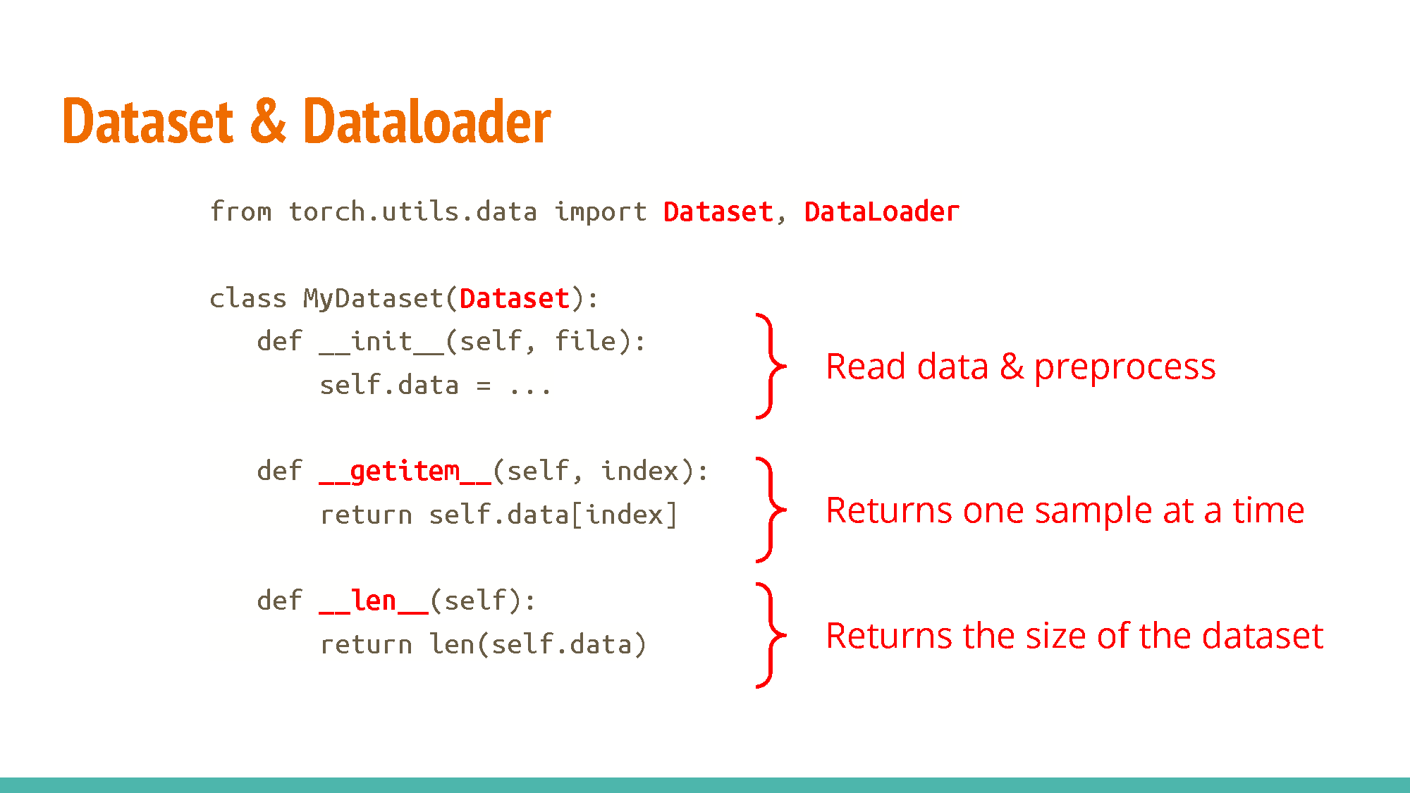
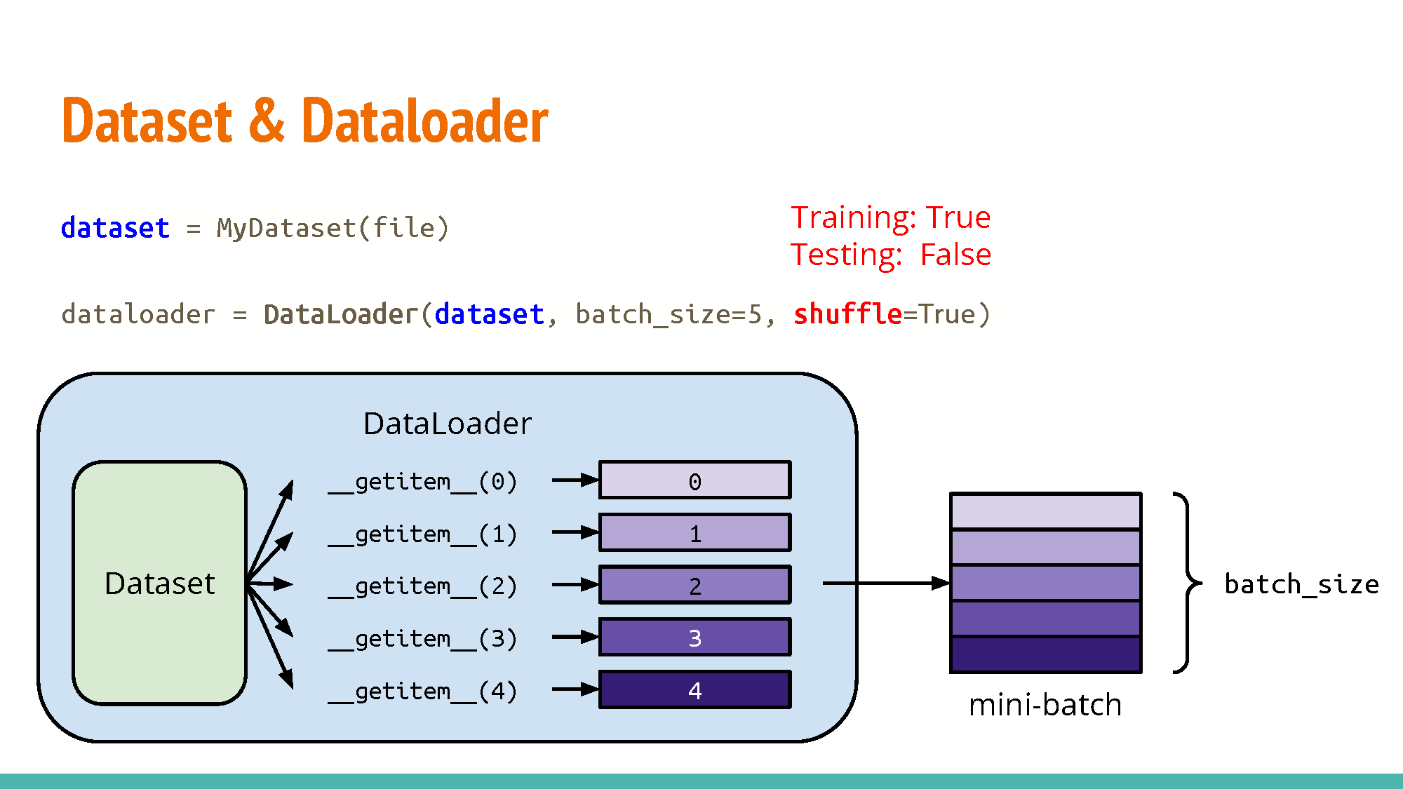
Training

Define Neural Network:

Linear Layer (Fully-connected Layer)

torch.nn.Linear(in_features, out_features)

>>> layer = torch.nn.Linear(32, 64)
>>> layer.weight.shape
torch.Size([64, 32])
>>> layer.bias.shape
torch.Size([64])

Non-Linear Activation Function

torch.nn.Sigmoid()
torch.nn.ReLU()

import torch.nn as nn
           
class MyModel(nn.Module):
def __init__(self):
super().__init__()  # super(MyModel, self).__init__()
self.net = nn.Sequential(
nn.Linear(10, 32),
nn.Sigmoid(),
nn.Linear(32, 1)
)
def forward(self, x):
return self.net(x)

Loss Function:
- torch.nn.MSELoss() for regression
- torch.nn.CrossEntropyLoss() for classification
```
criterion = nn.MSELoss()
loss = criterion(model_output, expected_value)
```
Optimization:
- torch.optim.SGD(model.parameters(), lr, momentum=0)
- torch.optim.Adam()
```
optimizer = torch.optim.SGD(model.parameters(), lr, momentum=0)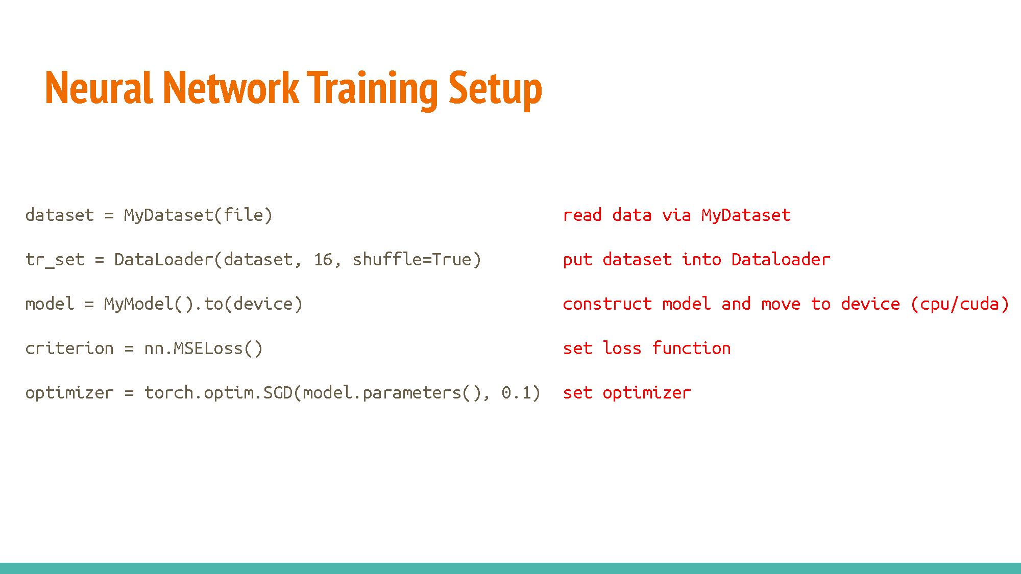
```

For every batch of data:

Call optimizer.zero_grad() to reset gradients of model parameters.
Call loss.backward() to backpropagate gradients of prediction loss.
Call optimizer.step() to adjust model parameters.

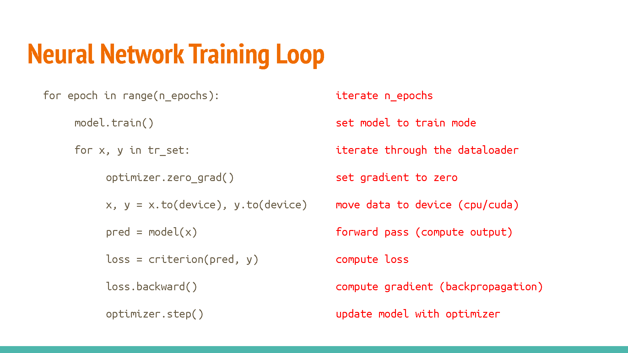
Validation

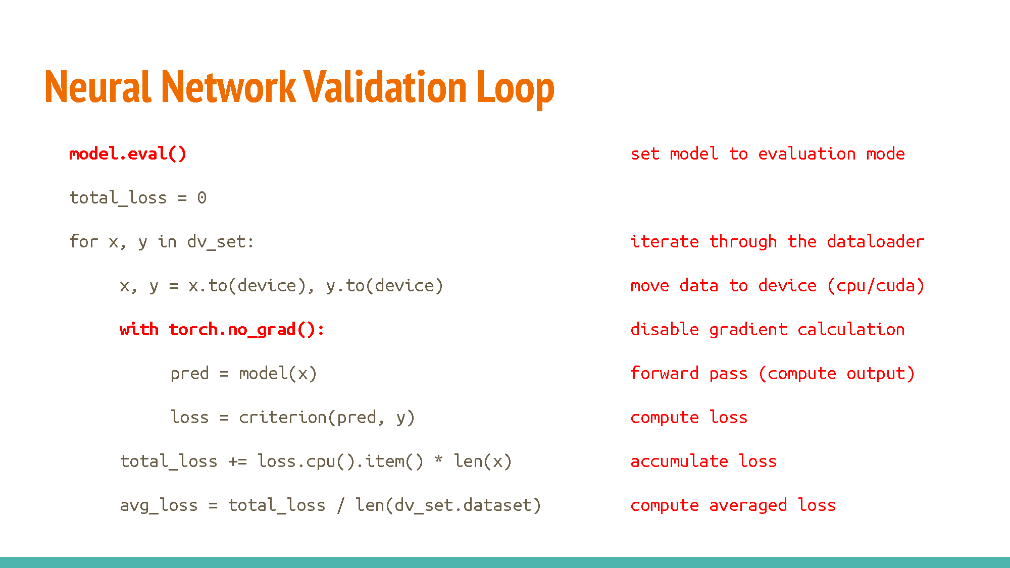
Testing

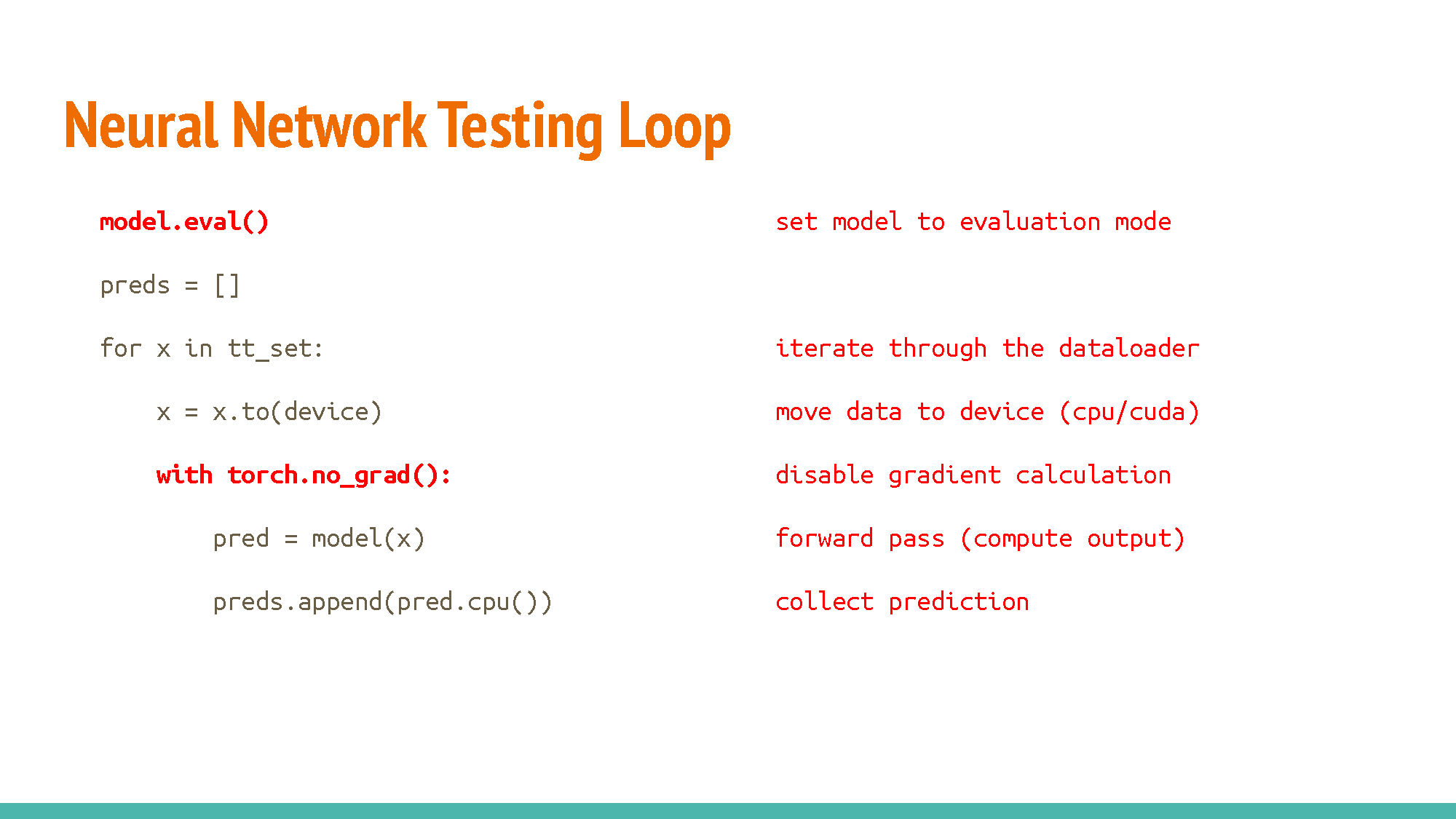
Save/Load Trained Models

Save
```
torch.save(model.state_dict(), path)
```

Load

ckpt = torch.load(path)  # checkpoint
model.load_state_dict(ckpt)

torchvision
torchaudio
torchtext
Huggingface Transformers
Fairseq
torchdrug

Common Errors

When the shape of a tensor is incorrect, use transpose, squeeze, unsqueeze to align the dimensions.

TensorBoard

VSCode: Terminal tensorboard --logdir runs

Colab

use % instead of ! for cd command

连接到自己的Google Drive

from google.colab import drive
drive.mount('/content/drive')

Colab保持运行：方法

Libraries

PyTorch / TensorFlow

Hugging Face

PyG / DGL / DIG / NetworkX / DGL/DGL-lifesci

Captum / SHAP

scikit-learn

NumPy / Pandas / Matplotlib / Seaborn / Plotly

RDKit / DeepChem

Hyperopt/Optuna

learn2learn / Awesome-META+

Flask / Streamlit / FastAPI

《深度学习入门-斋藤康毅》P171 ↩